Discriminant analysis is a very important statistical tool used by researchers throughout. It helps in enhancing or deriving conclusions out of raw data.It is slightly complicated in parts but on the whole it gives good analytical results.
Discriminant analysis is a statistical method that is used by researchers to help them understand the relationship between a "dependent variable" and one or more "independent variables." A dependent variable is the variable that a researcher is trying to explain or predict from the values of the independent variables. Discriminant analysis is similar to regression analysis and analysis of variance (ANOVA). The principal difference between discriminant analysis and the other two methods is with regard to the nature of the dependent variable.
Discriminant analysis requires the researcher to have measures of the dependent variable and all of the independent variables for a large number of cases. In regression analysis and ANOVA, the dependent variable must be a "continuous variable." A numeric variable indicates the degree to which a subject possesses some characteristic, so that the higher the value of the variable, the greater the level of the characteristic. A good example of a continuous variable is a person's income.
In discriminant analysis, the dependent variable must be a "categorical variable."
The values of a categorical variable serve only to name groups and do not necessarily indicate the degree to which some characteristic is present. An example of a categorical variable is a measure indicating to which one of several different market segments a customer belongs; another example is a measure indicating whether or not a particular employee is a "high potential" worker. The categories must be mutually exclusive; that is, a subject can belong to one and only one of the groups indicated by the categorical variable. While a categorical variable must have at least two values (as in the "high potential" case), it may have numerous values (as in the case of the market segmentation measure). As the mathematical methods used in discriminant analysis are complex, they are described here only in general terms. We will do this by providing an example of a simple case in which the dependent variable has only two categories.
Discriminant analysis is most often used to help a researcher predict the group or category to which a subject belongs. For example, when individuals are interviewed for a job, managers will not know for sure how job candidates will perform on the job if hired. Suppose, however, that a human resource manager has a list of current employees who have been classified into two groups: "high performers" and "low performers." These individuals have been working for the company for some time, have been evaluated by their supervisors, and are known to fall into one of these two mutually exclusive categories. The manager also has information on the employees' backgrounds: educational attainment, prior work experience, participation in training programs, work attitude measures, personality characteristics, and so forth. This information was known at the time these employees were hired. The manager wants to be able to predict, with some confidence, which future job candidates are high performers and which are not. A researcher or consultant can use discriminant analysis, along with existing data, to help in this task.
There are two basic steps in discriminant analysis. The first involves estimating coefficients, or weighting factors, that can be applied to the known characteristics of job candidates (i.e., the independent variables) to calculate some measure of their tendency or propensity to become high performers. This measure is called a "discriminant function." Second, this information can then be used to develop a decision rule that specifies some cut-off value for predicting which job candidates are likely to become high performers.
The tendency of an individual to become a high performer can be written as a linear equation. The values of the various predictors of high performer status (i.e., independent variables) are multiplied by "discriminant function coefficients" and these products are added together to obtain a predicted discriminant function score. This score is used in the second step to predict the job candidates likelihood of becoming a high performer. Suppose that you were to use three different independent variables in the discriminant analysis. Then the discriminant function has the following form:
where D = discriminant function score,
B , = discriminant function coefficient relating independent variable i to the discriminant function score,
X = value of independent variable i.
The equation is quite similar to a regression equation. Conventional regression analysis should not be used in place of discriminant analysis. The dependent variable would have only two values (high performer and low performer) and would thus violate important assumptions of the regression model. Discriminant analysis does not have these limitations with respect to the dependent variable.
Estimation of the discriminant function coefficients requires a set of cases in which values of the independent variables and the dependent variables are known. In the case described above, the company has this information for a current group of employees. There are several different ways that can be used to estimate discriminant function coefficients, but all work on the same general principle: the values of the coefficients are selected so that differences between the groups defined by the dependent variable are maximized with regard to some objective function. One commonly used objective function is the F-ratio, which is defined as it is in ANOVA and regression problems. The coefficients are chosen to maximize the F-ratio when analysis of variance is performed on the resulting discriminant function, using the dependent variable (i.e., job performance) as the grouping variable. Most general statistical programs, such as the Statistical Package for the Social Sciences, contain discriminant analysis modules.
There are various tests of significance that can be used in discriminant analysis. One widely used test statistic is based on Wilks lambda, which provides an assessment of the discriminating power of the function derived from the analysis. If this value is found to be statistically significant, then the set of independent variables can be assumed to differentiate between the groups of the categorical variable. This test, which is analogous to the F-ratio test in ANOVA and regression, is useful in evaluating the overall adequacy of the analysis.
Unfortunately, discriminant analysis does not generate estimates of the standard errors of the individual coefficients, as in regression, so it is not quite so simple to assess the statistical significance of each coefficient. For example, most discriminant analysis programs have a stepwise option. Independent variables are entered into the equation one at a time. Again, Wilks lambda can be used to assess the potential contribution of each variable to the explanatory power of the model. Variables from the set of independent variables are added to the equation until a point is reached for which additional items provide no statistically significant increment in explanatory power.
Once the analysis is completed, the discriminant function coefficients can be used to assess the contributions of the various independent variables to the tendency of an employee to be a high performer. The discriminant function coefficients are analogous regression coefficients and they range between values of -1.0 and 1.0. The first box in Figure 1 (on the facing page) provides hypothetical results of the discriminant analysis. The second box provides the within-group averages for the discriminant function for the two categories of the dependent variable. Note that the high performers have an average score of 1.45 on the discriminant function, while the low performers have an average score of -.89. The discriminant function is treated as a standardized variable, so it has a mean of zero and a standard deviation of one. The average values of the discriminant function scores are meaningful only in that they help us interpret the coefficients. Since the high performers are at the upper end of the scale, all of the positive coefficients indicate that the greater the value of those variables, the greater the likelihood of a worker being a high performer (e.g., education, motivation). The magnitudes of the coefficients also tell us something about the relative contributions of the independent variables. The closer the value of a coefficient is to zero, the weaker it is as a predictor of the dependent variable. On the other hand, the closer the value of a coefficient is to either 1.0 or -1.0, the stronger it is as a predictor of the dependent variable. In this example, then, years of education and ability to handle stress both have positive coefficients, though the latter is quite weak. Finally, individuals who place high importance on family life are less likely to be high performers than those who do not.
The second step in discriminant analysis involves predicting to which group in the dependent variable a particular case belongs. A subject's discriminant score can be translated into a probability of being in a particular group by means of Bayes Rule. Separate probabilities are computed for each group and the subject is assigned to the group with the highest probability. Another test of the adequacy of a model is the degree to which known cases are correctly classified. As in other statistical procedures, it is generally preferable to test the model on a set of cases that were not used to estimate the model's parameters. This provides a more conservative test of the model. Thus, a set of cases should, if possible, be saved for this purpose. Having completed the analysis, the results can be used to predict the work potential of job candidates and hopefully serve to improve the selection process.
There are more complicated cases, in which the dependent variable has more than two categories. For example, workers might have been divided into three groups: high performers, average performers, low performers. Discriminant analysis allows for such a case, as well as many more categories. The interpretation, however, of the discriminant function scores and coefficients becomes more complex. The books included in the "Further Reading" section below explain in detail how to perform discriminant analysis with multiple categories and provide in-depth technical discussions.
KAPIL SHARMA
12087
MARKETING (2009-11)
6.2.11


Garima Singh 12081
23/1/11
The introduction session of BI-Workshop was very loaded inspite being an introductory session but it was definitely a very good session. The data looked never so good, meaningful and colourful.
We started with First Level Analysis where we were taught how to calculate Frequencies with the given data sheet. Then we covered Cross Tabulation both for 2 variables as well as 3 variables.
The third and the last technique for the day was Cluster Analysis in which two different types of clusters were covered- Divisive and Agglomerative, both these are types of Hierarchical Cluster.
Hierarchy type of cluster is done for Variables provided the number of objects is less than 50. K-Means type of cluster is done for Cases provided the number of objects is more than 50.
24/1/11
The second session was more relaxed. We started Perceptual Mapping a.k.a PerMap.
PerMap is of two types- Overall Similarity and Attribute Based. In Overall Similarity a thorough knowledge is required what goes in people's minds because of which they think two particular objects are similar/dissimilar. One disadvantage is that the hidden attributes might get exposed.
In Attribute-Based PerMap attributes are provided which gives rise to one major disadvantage, it being the chance missing of an important attribute.
We then learned how to make a PerMap in both the types in two as well as three dimensions and also the significance of Objective Function Value which is nothing but an error and how it gets reduced when PerMap display is changed from Two dimention to Three dimension.
25/1/11
The concluding session was on Factor Analysis wherein we learned how to divide a whole lot of given factors can be divided and then using factor
analysis (extraction method) less important factors can be eliminated.
Z-Scores were also covered in the last session of the workshop where one of the major things that we observed was that the graph of the variable (particularly Horse Power) was similar to the Z-Scores for Horse Power.
Thanks,
Garima Singh
The introduction session of BI-Workshop was very loaded inspite being an introductory session but it was definitely a very good session. The data looked never so good, meaningful and colourful.
We started with First Level Analysis where we were taught how to calculate Frequencies with the given data sheet. Then we covered Cross Tabulation both for 2 variables as well as 3 variables.
The third and the last technique for the day was Cluster Analysis in which two different types of clusters were covered- Divisive and Agglomerative, both these are types of Hierarchical Cluster.
Hierarchy type of cluster is done for Variables provided the number of objects is less than 50. K-Means type of cluster is done for Cases provided the number of objects is more than 50.
24/1/11
The second session was more relaxed. We started Perceptual Mapping a.k.a PerMap.
PerMap is of two types- Overall Similarity and Attribute Based. In Overall Similarity a thorough knowledge is required what goes in people's minds because of which they think two particular objects are similar/dissimilar. One disadvantage is that the hidden attributes might get exposed.
In Attribute-Based PerMap attributes are provided which gives rise to one major disadvantage, it being the chance missing of an important attribute.
We then learned how to make a PerMap in both the types in two as well as three dimensions and also the significance of Objective Function Value which is nothing but an error and how it gets reduced when PerMap display is changed from Two dimention to Three dimension.
25/1/11
The concluding session was on Factor Analysis wherein we learned how to divide a whole lot of given factors can be divided and then using factor
analysis (extraction method) less important factors can be eliminated.
Z-Scores were also covered in the last session of the workshop where one of the major things that we observed was that the graph of the variable (particularly Horse Power) was similar to the Z-Scores for Horse Power.
Thanks,
Garima Singh
Factor Analysis
Factor Analysis
When trying to explain something via measuring a range of independent variables, factor analysis helps reduce the number of reported variables by determining significant variables and 'combining' these into a a single variable. It may be used in this way either to discover factors or to test a hypothesis that they exist.
The determination is statistical, but the output is a 'virtual' or unobserved variable which combines the measured variables in a linear formula which combines observed measurements with 'factor loading' constant numbers.
Factor Analysis also can be used to help demonstrate how a complex measurement instrument is really measuring one or a few bigger things.
Perhaps the most well-known result of factor analysis is 'IQ', which is a 'virtual' variable based on variable measurements of ability in mathematics, language and logic.
Factor Analysis originated in psychometrics by Charles Spearman (as in Spearman correlation) and Raymond Cattell (as in 16PF) with the assessment of intelligence and personality, and has since spread to many other fields, from marketing to operations research.
Factor Analysis is different to much research, which focuses on the relationships between independent and dependent variables. In contrast, Factor Analysis focuses on the relationship between multiple independent variables. 'Factor' basically means 'independent variable', although in this case the 'factors' are the new 'virtual' variables.
The use of Factor Analysis and its results is often an imprecise science and hence subject to debate (for example 'IQ' has been heavily criticized). Nevertheless it provides a simplification process that in practice can be very useful.
Principal component analysis
Principal Component Analysis is a variant of Factor Analysis and is equivalent when model 'errors' have the same variance. The difference lies in how Principal Component Analysis uses the total variance in the data and assume linear variable combinations, whilst Common Factor Analysis uses the common variance in the data and assumes latent variables.
Principal Component Analysis constructs as many components as there are original variables. The first component takes into account the greatest amount of variance between the variables, giving the weighting of these variables to form the single component. The second component is constructed to account for as much variance is left over that is not accounted for by the first component. The third component accounts for variance not accounted for by the first two components, and so on.
Normally, the first component is much larger than the rest, with a rapid drop off through the second and third components. If there is no useful way of reducing the matrix of variable correlations into a smaller number of factors then all components will be approximately equal.
Eigenvalues
Eigenvalues represent the proportion of variance explained by a given variable. With five variables, the sum of the eigenvalues will be 5. Sorting the factors by eigenvalue thus results in the first factor having the greatest importance (explaining the greatest amount of variance).
Eigenvalues can be used to help select the factors to select and carry forward for future use. Ways of doing this include:
· Greater than one: Select variables where the eigenvalue is >1.
· Fixed number: Select the top N variables only.
· Proportion explained: Select a proportion of variance that you want to explain, say 95%, then select those variables that fit within this.
· A Scree Plot is a simple sorted graph of Eigenvalues and can be used to select variables by taking only those on the steep part of the curve.
Orthogonal rotation
Factors selected through eigenvalue analysis may be refined further through orthogonal rotation. 'Orthogonal' factors are metaphorically at 'right angles' to one another, which means they do not correlate with one another and are so even more independent, making them useful measures.
For example if you were measuring types of intelligence, it would help if, say, creative intelligence was completely different from mathematical intelligence, so if you were working on one it would not 'leak' over into another area.
Vivek Kumar Singh
MBA – Operations Group 11
Discriminant Function Analysis
Discriminant Function Analysis
The main purpose of a discriminant function analysis is to predict group membership based on a linear combination of the interval variables. The procedure begins with a set of observations where both group membership and the values of the interval variables are known. The end result of the procedure is a model that allows prediction of group membership when only the interval variables are known. A second purpose of discriminant function analysis is an understanding of the data set, as a careful examination of the prediction model that results from the procedure can give insight into the relationship between group membership and the variables used to predict group membership.
For example, a graduate admissions committee might divide a set of past graduate students into two groups: students who finished the program in five years or less and those who did not. Discriminant function analysis could be used to predict successful completion of the graduate program based on GRE score and undergraduate grade point average. Examination of the prediction model might provide insights into how each predictor individually and in combination predicted completion or non-completion of a graduate program.
Another example might predict whether patients recovered from a coma or not based on combinations of demographic and treatment variables. The predictor variables might include age, sex, general health, time between incident and arrival at hospital, various interventions, etc. In this case the creation of the prediction model would allow a medical practitioner to assess the chance of recovery based on observed variables. The prediction model might also give insight into how the variables interact in predicting recovery.
The simplest case of discriminant function analysis is the prediction of dichotomous group membership based on a single variable. An example of the simplest case is the prediction of successful completion of a graduate program based on the GRE verbal score. In this case, since the prediction model includes only a single variable, it gives little insight into how variables interact with each other in prediction. Thus prediction of group membership will be the major focus of the next section of this chapter.
With respect to the data file and purpose of analysis, this simplest case is identical to the case of linear regression with dichotomous dependent variables. As discussed previously, data of this type may be represented in any number of different forms: scatterplots, tables of means and standard deviations, and overlapping frequency polygons. Because overlapping frequency polygons have such an intuitive appeal, they will be used to describe how discriminant function analysis works.
A single interval variable might discriminate between groups in an almost perfect fashion, not at all, or somewhere in between. For example, if one wished to differentiate adult males and females, one could collect information on how many bras the person owned, score on the last statistics test, and height. In the case of the number of bras, the discrimination would be very good, but not perfect (some women don't own any bras, some men do). In the case of the score on the last statistics test, little discrimination would be possible because males and females generally score about the same. In the case of height, some discrimination between adult males and females would be possible, but it would be far from perfect.
In general, the larger the difference between the means of the two groups relative to the within groups variability, the better the discrimination between the groups. The following program allows the student to explore data sets with different degrees of discrimination ability.
Navneet Kumar
MBA -operations Group 11
Major Clustering Methods Explained with it Physical Significance in Statistics
Blog By: Milind Suryavanshi_Operations_Group 11_ (Roll No. 12031)
Major Clustering Methods Explained with it Physical Significance in Statistics
A Categorization of Major Clustering Methods
- Partitioning method. It classifies the data into k groups, which together satisfy the following requirements: (1) each group must contain at least one object, and (2) each object must belong to exactly one group. Like the algorithms k-means and k-medoids. The cons of it is, most partitioning methods cluster objects based on the distance between objects. Such methods can find only spherical-shaped clusters and encounter difficulty at discovering clusters of arbitrary shapes.
- Hierarchical methods. A hierarchical method creates a hierarchical decomposition of the given set of data objects. Hierarchical methods suffer from the fact that once a step (merge or split) is done, it can never be undone.
- Density-based methods. The general idea is to continue growing the given cluster as long as the density (number of objects or data points) in the “neighborhood” exceeds some threshold; that is, for each data point within a given cluster, the neighborhood of a given radius has to contain at least a minimum number of points. Such a method can be used to filter out noise (outliers) and discover clusters of arbitrary shape.
- Grid-based methods. Grid-based methods quantize the object space into a finite number of cells that form a grid structure. The main advantage of this approach is its fast processing time, which is typically independent of the number of data objects and dependent only on the number of cells in each dimension in the quantized space.
- Model-based methods. Model-based methods hypothesize a model for each of the clusters and find the best fit of the data to the given model. A model-based algorithm may locate clusters by constructing a density function that reflects the spatial distribution of the data points.
- Other special method.
- Clustering high-dimensional data
- Constraint-based clustering
Given D, a data set of n objects, and k, the number of clusters to form, a partitioning algorithm organizes the objects into k partitions (k ≤ n), where each partition represents a cluster. The usually used methods are k-Means and k-Medoids.
The k-means algorithm takes the input parameter, k, and partitions a set of n objects into k clusters so that the resulting intracluster similarity is high but the intercluster similarity is low. Cluster similarity is measured in regard to the mean value of the objects in a cluster, which can be viewed as the cluster’s centroid or center of gravity.
It proceeds as follows:
1 Randomly selects k of the objects, each of which initially represents a cluster mean or center.
2 For each of the remaining objects, an object is assigned to the cluster to which it is the most similar, based on the distance between the object and the cluster mean.
3 It then computes the new mean for each cluster. This process iterates until the criterion function converges. Typically, the square-error criterion is used, defined as
where E is the sum of the square error for all objects in the data set; p is the point in space representing a given object; and mi is the mean of cluster Ci (both p and m_i are multidimensional). In other words, for each object in each cluster, the distance from the object to its cluster center is squared, and the distances are summed.
4 Iterate this process until no change happens.
The pros of this method:
- It works well when the clusters are compact clouds that are rather well separated from one another.
- The method is relatively scalable and efficient in processing large data sets because the computational complexity of the algorithm is O(nkt), where n is the total number of objects, k is the number of clusters, and t is the number of iterations.
- The method often terminates at a local optimum
The cons of this method:
- It can be applied only when the mean of a cluster is defined. This may not be the case in some applications.
- It need users to specify k.
- It is not suitable for discovering clusters with nonconvex shapes or clusters of very different size.
- It is sensitive to noise and outlier data points because a small number of such data can substantially influence the mean value.
- Often terminates at local optimal
Hierarchical clustering methods can be further classified as either agglomerative or divisive, depending on whether the hierarchical decomposition is formed in a bottom-up (merging) or top-down (splitting) fashion. The quality of a pure hierarchical clustering method suffers fromits inability to performadjustment once amerge or split decision has been executed. That is, if a particular merge or split decision later turns out to have been a poor choice, the method cannot backtrack and correct it.
Four widely used measures for distance between clusters are as follows, where |p-p'| is the distance between two objects or points, p and p'; m_ is the mean for cluster,C_i; and n_i is the number of objects in C_i.
Note: Refer to Image at the reference provided
One promising direction for improving the clustering quality of hierarchical methods is to integrate hierarchical clustering with other clustering techniques, resulting in multiple-phase clustering.
BIRCH is designed for clustering a large amount of numerical data by integration of hierarchical clustering (at the initial microclustering stage) and other clustering methods such as iterative partitioning (at the later macroclustering stage). It overcomes the two difficulties of agglomerative clustering methods: (1) scalability and (2) the inability to undo what was done in the previous step.
ROCK (RObust Clustering using linKs) is a hierarchical clustering algorithm that explores the concept of links (the number of common neighbors between two objects) for data with categorical attributes.
Two distinct clusters may have a few points or outliers that are close; therefore, relying on the similarity between points to make clustering decisions could cause the two clusters to be merged. ROCK takes a
more global approach to clustering by considering the neighborhoods of individual pairs of points. If two similar points also have similar neighborhoods, then the two points likely belong to the same cluster and so can be merged.
Chameleon is a hierarchical clustering algorithm that uses dynamic modeling to determine the similarity between pairs of clusters. In Chameleon, cluster similarity is assessed based on how well-connected objects are within a cluster and on the proximity of clusters. That is, two clusters are merged if their interconnectivity is high and they are close together.
Chameleon has been shown to have greater power at discovering arbitrarily shaped clusters of high quality than several well-known algorithms such as BIRCH and densitybased DBSCAN. However, the processing cost for high-dimensional data may require O(n2) time for n objects in the worst case.
To discover clusters with arbitrary shape, density-based clustering methods have been developed. These typically regard clusters as dense regions of objects in the data space that are separated by regions of low density (representing noise).
DBSCAN (Density-Based Spatial Clustering of Applications with Noise) is a density based clustering algorithm. The algorithm grows regions with sufficiently high density into clusters and discovers clusters of arbitrary shape in spatial databases with noise. It defines a cluster as a maximal set of density-connected points.
A density-based cluster is a set of density-connected objects that is maximal with respect to density-reachability. Every object not contained in any cluster is considered to be noise.
This method is sensitive to its parameter e and MinPts, and leaves the user with the responsibility of selecting parameter values that will lead to the discovery of acceptable clusters.
If a spatial index is used, the computational complexity of DBSCAN is O(nlogn), where n is the number of database objects. Otherwise, it is O(n2).
OPTICS computes an augmented cluster ordering for automatic and interactive cluster analysis.
Because of the structural equivalence of the OPTICS algorithm to DBSCAN, the OPTICS algorithm has the same runtime complexity as that of DBSCAN, that is, O(nlogn) if a spatial index is used, where n is the number of objects.
DENCLUE (DENsity-based CLUstEring) is a clustering method based on a set of density distribution functions. The method is built on the following ideas: (1) the influence of each data point can be formally modeled using a mathematical function, called an influence function, which describes the impact of a data point within its neighborhood; (2) the overall density of the data space can be modeled analytically as the sum of the influence function applied to all data points; and (3) clusters can then be determined mathematically by identifying density attractors, where density attractors are local maxima of the overall density function.
The major advantages DENCLUE has are
- It has a solid mathematical foundation and generalizes various clustering methods, including partitioning, hierarchical, and density-based methods;
- It has good clustering properties for data sets with large amounts of noise;
- It allows a compact mathematical description of arbitrarily shaped clusters in highdimensional data sets;
- It uses grid cells, yet only keeps information about grid cells that actually contain data points. It manages these cells in a tree-based access structure, and thus is significantly faster than some influential algorithms, such as DBSCAN.
However, the method requires careful selection of the density parameter and noise threshold, as the selection of such parameters may significantly influence the quality of the clustering results.
The grid-based clustering approach uses a multiresolution grid data structure. It quantizes the object space into a finite number of cells that form a grid structure on which all of the operations for clustering are performed. The main advantage of the approach is its fast processing time, which is typically independent of the number of data objects, yet dependent on only the number of cells in each dimension in the quantized space.
STING is a grid-based multiresolution clustering technique in which the spatial area is divided into rectangular cells. There are usually several levels of such rectangular cells corresponding to different levels of resolution, and these cells form a hierarchical structure: each cell at a high level is partitioned to form a number of cells at the next lower level. Statistical information regarding the attributes in each grid cell (such as the mean, maximum, and minimum values).
STING offers several advantages: (1) the grid-based computation is query-independent, because the statistical information stored in each cell represents the summary information of the data in the grid cell, independent of the query; (2) the grid structure facilitates parallel processing and incremental updating; and (3) the method’s efficiency is a major advantage: STING goes through the database once to compute the statistical parameters of the cells, and hence the time complexity of generating clusters is O(n), where n is the total number of objects. After generating the hierarchical structure, the query processing time is O(g), where g is the total number of grid cells at the lowest level, which is usually much smaller than n.
WaveCluster is a multiresolution clustering algorithm that first summarizes the data by imposing a multidimensional grid structure onto the data space. It then uses a wavelet transformation to transformthe original feature space, finding dense regions in the transformed space.
11. Model-Based Clustering Methods
Model-based clustering methods attempt to optimize the fit between the given data and some mathematical model. Such methods are often based on the assumption that the data are generated by a mixture of underlying probability distributions.
Conceptual clustering is a form of clustering in machine learning that, given a set of unlabeled objects, produces a classification scheme over the objects. Unlike conventional clustering, which primarily identifies groups of like objects, conceptual clustering goes one step further by also finding characteristic descriptions for each group, where each group represents a concept or class. Hence, conceptual clustering is a two-step process: clustering is performed first, followed by characterization. Here, clustering quality is not solely a function of the individual objects. Rather, it incorporates factors such as thegenerality and simplicity of the derived concept descriptions.
Most methods of conceptual clustering adopt a statistical approach that uses probability measurements in determining the concepts or clusters. Probabilistic descriptions are typically used to represent each derived concept.
13. Clustering High-Dimensional Data
Most clusteringmethods are designed for clustering low-dimensional data and encounter challenges when the dimensionality of the data grows really high. This is because when the dimensionality increases, usually only a small number of dimensions are relevant to certain clusters, but data in the irrelevant dimensions may producemuch noise and mask the real clusters to be discovered.Moreover, when dimensionality increases, data usually become increasingly sparse because the data points are likely located in different dimensional subspaces.
To overcome this difficulty, we may consider using feature (or attribute) transformation and feature (or attribute) selection techniques. Feature transformation methods, such as principal component analysis and singular value decomposition, transformthe data onto a smaller space while generally preserving the original relative distance between objects. They summarize data by creating linear combinations of the attributes, and may discover hidden structures in the data. However, such techniques do not actually remove any of the original attributes from analysis. This is problematic when there are a large number of irrelevant attributes. The irrelevant information may mask the real clusters, even after transformation. Moreover, the transformed features (attributes) are often difficult to interpret, making the clustering results less useful. Thus, feature transformation is only suited to data sets where most of the dimensions are relevant to the clustering task. Unfortunately, real-world data sets tend to have many highly correlated, or redundant, dimensions.
Another way of tackling the curse of dimensionality is to try to remove some of the dimensions. Attribute subset selection (or feature subset selection7) is commonly used for data reduction by removing irrelevant or redundant dimensions (or attributes). Given a set of attributes, attribute subset selection finds the subset of attributes that are most relevant to the data mining task. Attribute subset selection involves searching through various attribute subsets and evaluating these subsets using certain criteria. It is most commonly performed by supervised learning—the most relevant set of attributes are found with respect to the given class labels. It can also be performed by an unsupervised process, such as entropy analysis, which is based on the property that entropy tends to be low for data that contain tight clusters.
Other evaluation functions, such as category utility, may also be used. Subspace clustering is an extension to attribute subset selection that has shown its strength at high-dimensional clustering. It is based on the observation that different subspaces may contain different, meaningful clusters. Subspace clustering searches for groups of clusters within different subspaces of the same data set. The problem becomes how to find such subspace clusters effectively and efficiently.
14. Constraint-Based Cluster Analysis
Users often have a clear view of the application requirements, which they would ideally like to use to guide the clustering process and influence the clustering results. Thus, in many applications, it is desirable to have the clustering process take user preferences and constraints into consideration.
One person’s noise could be another person’s signal. Outlier detection and analysis are very useful for fraud detection, customized marketing, medical analysis, and many other tasks. Computer-based outlier analysis methods typically followeither a statistical distribution-based approach, a distance-based approach, a density-based local outlier detection approach, or a deviation-based approach.
Blog By: Milind Suryavanshi_Operations_Group 11_ (Roll No. 12031)
Everything about Factor Analysis that you may want to Know!
Blog by- Milind Suryavanshi (Operations_Group 11_12031)
Everything about Factor Analysis that you may want to Know!
Note: Please refer to the references for the original work to view relevant tables/figures.
INTRODUCTION
Thousands of variables have been proposed to explain or describe the complex variety and interconnections of social and international relations. Perhaps an equal number of hypotheses and theories linking these variables have been suggested.1
The few basic variables and propositions central to understanding remain to be determined. The systematic dependencies and correlations among these variables have been charted only roughly, if at all, and many, if not most, can be measured only on presence-absence or rank order scales. And to take the data on any one variable at face value is to beg questions of validity, reliability, and comparability.
Confronted with entangled behavior, unknown interdependencies, masses of qualitative and quantitative variables, and bad data, many social scientists are turning toward factor analysis to uncover major social and international patterns.2 Factor analysis can simultaneously manage over a hundred variables, compensate for random error and invalidity, and disentangle complex interrelationships into their major and distinct regularities.
Factor analysis is not without cost, however. It is mathematically complicated and entails diverse and numerous considerations in application. Its technical vocabulary includes strange terms such as eigenvalues, rotate, simple structure, orthogonal, loadings, and communality. Its results usually absorb a dozen or so pages in a given report, leaving little room for a methodological introduction or explanation of terms. Add to this the fact that students do not ordinarily learn factor analysis in their formal training, and the sum is the major cost of factor analysis: most laymen, social scientists, and policy-makers find the nature and significance of the results incomprehensible.
The problem of communicating factor analysis is especially crucial for peace research. Scholars in this field are drawn from many disciplines and professions, and few of them are acquainted with the method. As our empirical knowledge of conflict processes, behavior, conditions, and patterns become increasingly expressed in factor analytic terms, those who need this knowledge most in order to make informed policy decisions may be those who are most deterred by the packaging. Indeed, they are unlikely to know that this knowledge exists.3
A conceptual map, therefore, is needed to guide the consumers of findings in conflict and international relations through the terminological obstacles and quantitative obstructions presented by factor studies. The aim of this paper is to help draw such a map. Specifically, the aim is to enhance the understanding and utilization of the results of factor analysis. Instead of describing how to apply factor analysis or discussing the mathematical model involved, I shall try to clarify the technical paraphernalia which may conceal important substantive data, propositions, or scientific laws.
By way of orientation, the first section of this paper will present a brief conceptual review of factor analysis. In the second section the scientific context of the method will be discussed. The major uses of factor analysis will be listed and its relation to induction and deduction, description and inference, causation and explanation, and classification and theory will be considered. To aid understanding, the third section will outline the geometrical and algebraic factor models, and thefourth section will define the factor matrices and their elements--the vehicles for presenting factor results. Since comprehending factor rotation is important for interpreting the findings, thefifth and final section is devoted to clarifying its significance.
A bibliography of factor analysis texts and applications to conflict and international relations is given in an appendix.
1. CONCEPTUAL OVERVIEW
Factor analysis is a means by which the regularity and order in phenomena can be discerned. As phenomena co-occur in space or in time, they are patterned; as these co-occurring phenomena are independent of each other, there are a number of distinct patterns. Patterned phenomena are the essence of workaday concepts such as "table," "chair," and "house," and--at a less trivial level--patterns structure our scientific theories and hypotheses. We associate a pattern of attitudes, for example, with businessmen and another pattern with farmers. "Economic development" assumes a pattern of characteristics, as does the concept of "communist political system." The notion of conflict itself embodies a pattern of elements, i.e., two or more parties and a perception of mutually exclusive or contradictory values or goals. And to mention phenomena that everyone talks about, weather also has its patterns.
What factor analysis does is this: it takes thousands and potentially millions of measurements and qualitative observations and resolves them into distinct patterns of occurrence. It makes explicit and more precise the building of fact-linkages going on continuously in the human mind.
Let us look at a concrete example. Table 1 presents information on fourteen nations for ten characteristics. The nations are selected to reflect major regional, political, economic, and cultural groupings; the characteristics reflect different facets of each nation, including domestic instability and foreign conflict. The table thus contains 14 X 10, or 140 pieces of information for 1955. Factor analysis addresses itself to this question: "What are the patterns of relationship among these data?"

These patterns can be viewed from two perspectives. One can look at the pattern of variation of nations across their characteristics, and then group the nations by their profile similarity. One might group together nations which are all high on GNP per capita, low on trade, high on power, etc. When applied to discern patterns of profile similarity of individuals, groups, or nations, the analysis is called Q-factor analysis.4
The regularity in the data of Table 1 can be looked at from a second perspective, however. The focus now is the patterns of variation of characteristics. In Table 1, for example, nations high on GNP per capita also appear low on trade and power. There is a regularity, therefore, in the nation values on these three characteristics, and this regularity is described as a pattern of variation. Many of our social concepts define such patterns. For example, the concept of 11 economic development" involves (among other things) GNP per capita, literacy, urbanization, education, and communication; it is a pattern because these characteristics are highly intercorrelated with each other. Factor analysis applied to delineate patterns of variation in characteristics is called R-factor analysis.5
What actual patterns of characteristics are revealed for the data in Table 1 by factor analysis?Figure 1 displays the four major kinds of regularity in the interrelationships between the characteristics: power, US voting agreement, foreign conflict, and international law. They involve, respectively, 27.6, 21.0, 16.2, and 15.3 percent of the variation6 in the 140 pieces of information in Table 1; added together, these patterns indicate that 80.1 percent of this information has an underlying regularity.
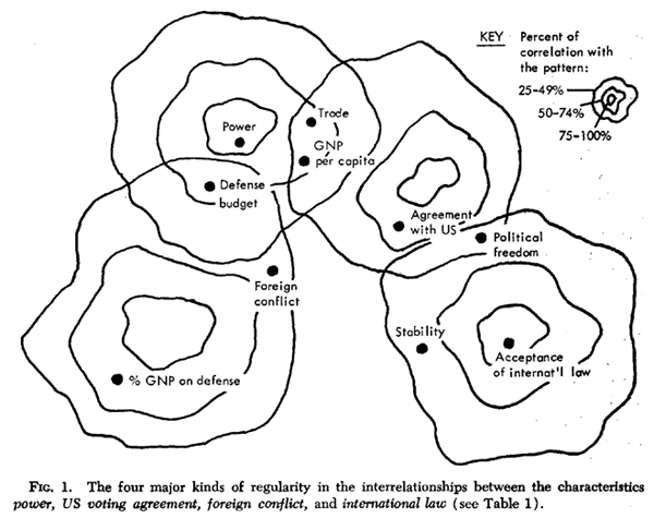
Each pattern in Figure 1 is laid out in three isobars. The central isobar includes characteristics with at least 75 percent of their variation involved in the pattern. These are most central to interpreting the pattern. The two remaining isobars define characteristics related to the pattern in the range of 50-74 percent and 25-49 percent of their variation, respectively. These groups of isobars show
- what patterns exist in the data and how they overlap,
- what characteristics are involved in what pattern and to what degree, and
- what characteristics are involved in more than one pattern.
To display another perspective, Figure 2 plots these four patterns as profiles for the nations inTable 1. On the horizontal axis, nations are ordered from low to high power pattern values. Magnitudes on the vertical axis are in standard scores, which is to say that the average score is zero and 95.5 percent of the fourteen nations will (if normally distributed) fall between scores of +2.00 and -2.00; 68.3 percent of them will fall between scores of +1.00 and -1.00. Each pattern has a different shape, which illustrates what is meant by saying that factor analysis divides the regularity in the data into its distinct patterns. If each of the ten characteristics in Table 1 were plotted as was done for the patterns in Figure 2, and those characteristics with similarly-shaped plots were grouped together, there would be four major groups, and the modal plot within each group would correspond to each of the patterns shown. Figure 1 and Figure 2 are alternativerepresentations of the results of factoring Table 1.

2. FACTOR ANALYSIS AND SCIENTIFIC METHOD
Factor analysis can be applied in order to explore a content area, structure a domain, map unknown concepts, classify or reduce data, illuminate causal nexuses, screen or transform data, define relationships, test hypotheses, formulate theories, control variables, or make inferences. Our consideration of these various overlapping usages will be related to several aspects of scientific method: induction and deduction; description and inference; causation, explanation, and classification; and theory.
This section will outline factor analysis applications relevant to various scientific and policy concerns. Many of the uses described below overlap. My aim is not to avoid redundancy but explicitly to relate factor analysis to the diverse interests of readers.
Interdependency and pattern delineation. If a scientist has a table of data--say, UN votes, personality characteristics, or answers to a questionnaire--and if he suspects that these data are interrelated in a complex fashion, then factor analysis may be used to untangle the linear relationships into their separate patterns. Each pattern will appear as a factor delineating a distinct cluster of interrelated data.
Parsimony or data reduction. Factor analysis can be useful for reducing a mass of information to an economical description. For example, data on fifty characteristics for 300 nations are unwieldy to handle, descriptively or analytically. The management, analysis, and understanding of such data are facilitated by reducing them to their common factor patterns. These factors concentrate and index the dispersed information in the original data and can therefore replace the fifty characteristics without much loss of information. Nations can be more easily discussed and compared on economic development, size, and politics dimensions, for example, than on the hundreds of characteristics each dimension involves.
Structure. Factor analysis may be employed to discover the basic structure of a domain. As a case in point, a scientist may want to uncover the primary independent lines or dimensions--such as size, leadership, and age--of variation in group characteristics and behavior. Data collected on a large sample of groups and factor analyzed can help disclose this structure.
Classification or description. Factor analysis is a tool for developing an empirical typology.7 It can be used to group interdependent variables into descriptive categories, such as ideology, revolution, liberal voting, and authoritarianism. It can be used to classify nation profiles into types with similar characteristics or behavior. Or it can be used on data matrices of a transaction type or a social-choice type to show how individuals, social groups, or nations cluster on their transactions with or choices of each other.
Scaling. A scientist often wishes to develop a scale on which individuals, groups, or nations can be rated and compared. The scale may refer to such phenomena as political participation, voting behavior, or conflict. A problem in developing a scale is to weight the characteristics being combined. Factor analysis offers a solution by dividing the characteristics into independent sources of variation (factors). Each factor then represents a scale based on the empirical relationships among the characteristics. As additional findings, the factor analysis will give the weights to employ for each characteristic when combining them into the scales. The factor score results (see Section 4.5 below) are actually such scales, developed by summing characteristics times these weights.
Hypothesis testing. Hypotheses abound regarding dimensions of attitude, personality, group, social behavior, voting, and conflict. Since the meaning usually associated with "dimension" is that of a cluster or group of highly intercorrelated characteristics or behavior, factor analysis may be used to test for their empirical existence. Which characteristics or behavior should, by theory, be related to which dimensions can be postulated in advance and statistical tests of significance can be applied to the factor analysis results.
Besides those relating to dimensions, there are other kinds of hypotheses that may be tested. To illustrate: if the concern is with a relationship between economic development and instability,holding other things constant, a factor analysis can be done of economic and instability variables along with other variables that may affect (hide, mediate, depress) their relationship. The resulting factors can be so defined (rotated) that the first several factors involve the mediating measures (to the maximum allowed by the empirical relationships). A remaining independent factor can be calculated to best define the postulated relationships between the economic and instability measures. The magnitude of involvement of both variables in this pattern enables the scientist to see whether an economic development-instability pattern actually exists when other things are held constant.
Data transformation. Factor analysis can be used to transform data to meet the assumptions of other techniques. For instance, application of the multiple regression technique assumes (if tests of significance are to be applied to the regression coefficients) that predictors--the so-called independent variables--are statistically unrelated (Ezekiel and Fox, 1959, pp. 283-84). If the predictor variables are correlated in violation of the assumption, factor analysis can be employed to reduce them to a smaller set of uncorrelated factor scores. The scores may be used in the regression analysis in place of the original variables, with the knowledge that the meaningful variation in the original data has not been lost.8 Likewise, a large number of dependent variables also can be reduced through factor analysis.
Exploration. In a new domain of scientific interest like peace research, the complex interrelations of phenomena have undergone little systematic investigation. The unknown domain may be explored through factor analysis. It can reduce complex interrelationships to a relatively simple linear expression and it can uncover unsuspected, perhaps startling, relationships. Usually the social scientist is unable to manipulate variables in a laboratory but must deal with the manifold complexity of behaviors in their social setting. Factor analysis thus fulfills some functions of the laboratory and enables the scientist to untangle interrelationships, to separate different sources of variation, and to partial out or control for undesirable influences on the variables of concern.9
Mapping. Besides facilitating exploration, factor analysis also enables a scientist to map the social terrain. By mapping I mean the systematic attempt to chart major empirical concepts and sources of variation. These concepts may then be used to describe a domain or to serve as inputs to further research. Some social domains, such as international relations, family life, and public administration, have yet to be charted. In some other areas, however, such as personality, abilities, attitudes, and cognitive meaning, considerable mapping has been done.
Theory. As will be discussed in Section 2.5 below, the analytic framework of social theories or models can be built from the geometric or algebraic structure of factor analysis.
The use of "and" rather than "versus" in the headings of this and the following subsection emphasizes that these different ways of interpreting or using factor analysis are not mutually exclusive. They are different sides of the same coin. The side evident in a particular set of results depends upon the interpretation.
Factor analysis is most familiar to researchers as an exploratory tool for unearthing the basic empirical concepts in a field of investigation. Representing patterns of relationship between phenomena, these basic concepts may corroborate the reality of prevailing concepts or may be so new and strange as to defy immediate labeling. Factor analysis is often used to discover such concepts reflecting unsuspected influences at work in a domain. The delineation of these interrelated phenomena enables generalizations to be made and hypotheses posed about the underlying influences bringing about the relationships. For example, if a political scientist were to factor the attributes and votes of legislators and were to find a pattern involving urban constituencies and liberal votes, he could use this finding to develop a theory linking urbanism and liberalism. The ability to relate data in a meaningful fashion is a prime aspect of induction and, for this, factor analysis is useful and efficient.
Factor analysis may also be employed deductively, in two ways. One way is to elaborate the geometric or algebraic structure of factor analysis as part of a theory. Within the theory the factor analysis model can then be used to arrive at deductions about phenomena. This approach is described more fully in Section 2.5 below.
The second deductive approach is to hypothesize the existence of particular dimensions and then to factor analyze the data to see whether these dimensions emerge.10 Although factor analysis is not often used this way, the restraint is not due to methodology but to research tradition. If, as an example, scholars believe that ideology, power, and trade are the primary patterns of international behavior, then this proposition can be tested. Data can be collected on those variables that index international relations in its greatest diversity, and those specific variables distinguishing (by theory) the ideology, power, and trade patterns should be defined. To test whether these patterns actually exist is the factor analysis task.
A data matrix alone may be of primary interest. Research is then centered on describing the regularities in these data. Statistical problems like the type of underlying frequency distribution, sample size, and randomness of selection are not part (and need not be part) of the research design. As cases in point, all roll call votes in a UN General Assembly session can be analyzed to describe the voting patterns of nations for that session, as did Alker (1964), or the voting blocs into which nations were grouped, as did Russett (1966).
Description may be only an intermediate goal, however. The ultimate goal may be to connect a number of descriptive studies to make generalizations about what patterns exist for such phenomena as, say, legislative voting, foreign conflict, political systems, personality, or role behavior.11 Although generalization from a number of descriptive studies is a form of inference, it need not be statistical inference in the sense that some statistical test of significance is applied. In fact, factor analysis is seldom employed for statistical inference, although many social scientists consider it a statistical method. The statistical requirement of a representative sample is usually met by the research design, but the additional statistical assumptions such as a normal frequency distribution are seldom satisfied. Indeed, the canonical factor model (Section 3 below) which has been formulated to allow statistical inference is seldom used, and tests of significance for factor loadings are virtually unknown in the applied literature.
Description, then, and generalization from a number of descriptive studies have been the tradition in applied factor analysis. Although tests of significance can be determined for the factors and loadings of a particular sample, factor analysis itself does not require such tests.12Factor analysis is a mathematical tool as is the calculus, and not a statistical technique like the chi-square, the analysis of variance, or sequential analysis.
2.4 Causation, Explanation, and Classification
The idea of "cause" has had a strange fascination for scientists. Books and scholarly papers have been devoted to just the meaning and usage of the term.13 No wonder, then, that the relationship between causation and factor analysis has been controversial in the factor analysis literature. The issue centers on whether a factor pattern represents a causal nexus.14
Modem science conceives of causation as a temporal regularity of phenomena or, more precisely, a functional (mathematical) relationship between phenomena. The term "cause" is then simply an expression of uniform relationships, that is, of a generally observed concurrence or concomitance of phenomena. Even though this interpretation drops out interesting connotations like "to bring about," or "to influence," it removes a fuzziness from the concept and gives it a denotation consonant with scientific method and philosophy.
Does factor analysis define factors, then, that can be called causes of the patterns they represent? The answer must be yes.15 Each of the variables analyzed is mathematically related to the factor patterns. The regularities in the phenomena are described by these patterns, and it is these regularities that indicate a causal nexus. just as the pattern of alignment of steel filings near a magnet can be described by the concept of magnetism, for example, so the concept of magnetism can be turned around and be said to cause the alignment. Likewise, an economic development pattern delineated by factor analysis can be called a cause. In this sense, a gregarious personality factor causes certain attitudes, a turmoil factor causes riots, and an urbanism factor causes liberal voting.
The term explanation adds nothing to the term cause. Although laden in the social sciences with a surplus meaning associated with verstehen, a feeling of understanding or getting the sense of something,16 the explanation of phenomena is nothing more than being able to predict or mathematically relate phenomena. To explain an event is to be able to predict it (see Hempel, 1965, Chapter 12 and, for contrast, Hanson, 1959). To explain that the Roman Empire fell because of disunity and moral decay is to say that, given the presence of these two elements in an empire with the characteristics of the Roman Empire, the empire will break up or be conquered.
Prediction itself is based on the identification of causal relations, i.e., regularity. Therefore, if a factor can be called a cause, it can be called an explanation.
If one wants to avoid controversy over causation, on the other band, factor patterns may be treated as purely descriptive or classificatory. A factor name like "turmoil" will then be a noun describing phenomena sharing one characteristic: appearance in time or space with a certain uniformity. "House," "horse," "social group," "legislature," and "nation" are such nouns, and factors may be conceived likewise. "Economic development" or "size," as factors actually delineated through factor analysis (Rummel, 1972), can be descriptive categories subsuming a pattern of telephones per capita, GNP per capita, and vehicles per capita as distinct from a pattern of population, area, and national income.
The aim of science is theory. Facts or data are meaningless in themselves. They must be linked through propositions which confer meaning. Were we unable to perceive such relationships, our capacity to manipulate, process, or understand facts would be overwhelmed. Relationships recurring with high probability become scientific laws that may be incorporated into a theory covering the domain in which they are applicable.
A scientific theory consists of two components:17 analytic and empirical. The analytic component is the linking of symbolic statements through chains of reasoning that obey logical or mathematical rules but that have little or no operational-empirical content. The symbols involved may refer to line, atom, dimension, force, power (mechanical or social), group, or ideology. Statements involving these symbols may be associated through verbal reasoning, symbolic logic, or mathematics. Whatever the symbols or mode of reasoning, this analytic component of theories can be the creation of the scientist's imagination, the distillation of a scholar's experience with the subject matter, or a tediously built structure slowly erected on a foundation of numerous experiments, investigation, and findings.
The empirical component of theories is operational. It fastens the abstract analytic part of a theory to the facts. While the analytic part need have no empirical interpretation, the empirical component must verifiably link to data for a theory to apply to "reality."
A confusion between the empirical and analytic parts of a theory may have militated against a more theoretical use of factor analysis. The geometric or algebraic nature of the factor model can structure the analytic framework of theory. The factors themselves can be postulated. From them, operational deductions with empirical content can be derived and tested.18
The factor model represents a mathematical formalism departing from the calculus functions of classical physics. The analytic part of the factor model is akin to that of quantum theory.19Vectors and their position, linear operators, and the dimensions (factors) of a system are the focus of concern.
Since factor analysis incorporates analytic possibilities as a theory and empirical techniques for connecting the theory to social phenomena, its potentiality promises much theoretical development for the social sciences. Looking ahead for a century, I suggest that factor analysis and the complementary multiple regression model are initiating a scientific revolution in the social sciences as profound and far-reaching as that initiated by the development of the calculus in physics.
3. THE FACTOR MODEL
In application, there are not one but several factor models which differ in significant respects. A model most often applied in psychology is called common factor analysis. Indeed, psychologists usually reserve the term "factor analysis" for just this model. Common factor analysis is concerned with defining the patterns of common variation among a set of variables. Variation unique to a variable is ignored. In contrast, another factor model called component factor analysis is concerned with patterning all the variation in a set of variables, whether common or unique.
Other factor models are image analysis, canonical analysis, and alpha analysis. Image analysis has the same purpose as common factor analysis, but more elegant mathematical properties. Canonical analysis defines common factors for a sample of cases that are the best estimates of those for the population; it enables tests of significance. Alpha analysis defines common factors for a sample of variables that are the best estimates of those in a universe of content.
It would be beyond the purpose of this paper to discuss these models in any detail. (For such a discussion, see Rummel, 1970, Chapter 5.) In the following sections only their general mathematical properties will be outlined. These properties clearly distinguish the factor analysis models from others used in the social sciences, such as analysis of variance and multiple regression, and justify our consideration of these properties in reference to a generalized factor model.
An understanding of the patterns defined by factor analysis can be enhanced through a geometric interpretation. Each nation of Table 1 can be thought of as defining a coordinate axis of a geometric space. For example, the US, the UK, and the USSR can define a three-dimensional space as given in Figure 3. Imagine that the axis for the UK is projecting at right angles from the paper. Although pictorially constrained to three dimensions, the space can be analytically extended to fourteen dimensions at right angles to each other and thus represent the fourteen nations in Table 1.
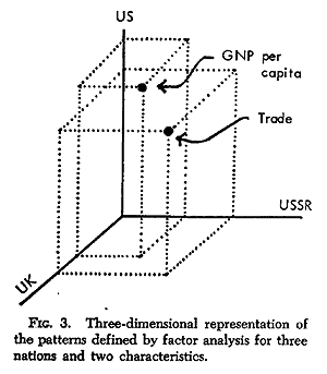
Now, in this space each characteristic can be considered a point located according to its value for each nation. Such a plot is shown in Figure 3 for the GNP per capita and trade values of the US, UK, and USSR. To make the plot explicit, projections for each point are drawn as dotted lines to each axis.20
If for each point in Figure 3 we draw a line from the origin to the point and top the line off with an arrowhead as shown in Figure 4, then we have a vector representation of the data. The ten characteristics of Table 1 similarly plotted as vectors in an imaginary space of the fourteen nations (dimensions) would describe a vector space. In this space, consider two vectors representing any two of these characteristics for the fourteen nations.
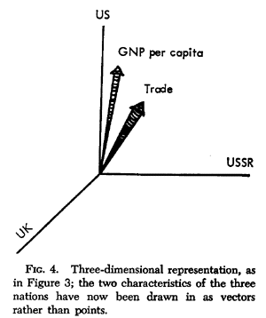
The angle between these vectors measures the relationship between the two characteristics for the fourteen nations. The closer to 90o the angle is, the less the relationship is. If two vectors are at a right angle, the characteristics they represent are uncorrelated: they have no relationship to each other. In other words, some nations will be high on one characteristic, say GNP per capita, and low on the other, say trade; some nations will be low on GNP per capita and high on trade; some nations will be high on both, and some will be low on both. No regularity exists in their covariation.
The closer the angle between the vectors is to zero, the stronger the relationship between the characteristics. An angle of zero means that nations high or low on one characteristic are proportionately high or low on the other. Obtuse angles mean a negative relationship. At the extreme, an angle of 180o between two vectors means that the two characteristics are inversely related: a nation high on one characteristic is proportionately low on the other.21
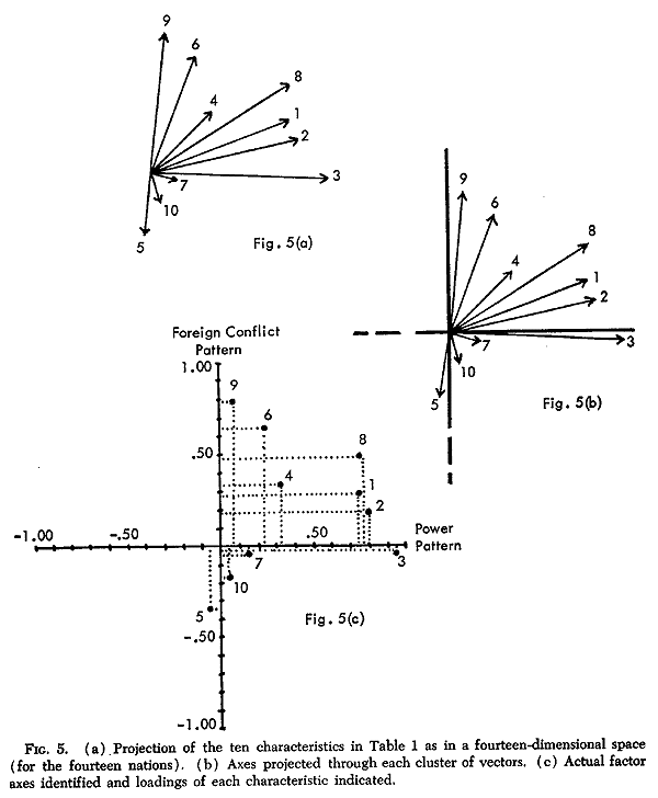
Let the ten characteristics of Table 1 be projected in the fourteen-dimensional space defined by the fourteen nations as suggested in Figure 5(a). The configuration of vectors will then reflect the data interrelationships. Characteristics that are highly interrelated will cluster together; characteristics that are unrelated will be at right angles to each other. By inspecting the configuration we can discern the distinct clusters of vectors (if such clusters exist), and these clusters index the patterns of relationship in the data: each cluster is a pattern.
Were we dealing with characteristics of two or three nations, patterns could be found by simply plotting the characteristics as vectors. What factor analysis does geometrically is this: it enables the clusters of vectors to be defined when the number of cases (dimensions) exceeds our graphical limit of three. Each factor delineated by factor analysis defines a distinct cluster of vectors.22
Consider Figure 5(a) again. Factor analysis would mathematically lay out such a plot and then project an axis through each cluster as shown in Figure 5(b). This is analogous to giving each vector point in a cluster a mass of one and letting the factor axes fall through their center of gravity.23 The projection of each vector point on the factor axes defines the clusters. These projections are called loadings and the factor axes are often called factors or dimensions.
Figure 5(c) pictures the power and foreign conflict patterns of Table 1. For simplicity, the configuration of points is shown, rather than vectors, and the two factor axes are indicated (as actually derived from a factor analysis). The loadings of each characteristic (i.e., each point in space) on each axis are also displayed. This figure may clarify how factor loadings as a set of numbers can define
- a pattern of relationships and
- the association of each characteristic with each pattern.
We will consider this geometrical perspective again when the factor matrices are described.
For the more symbolically oriented reader it may be helpful to present the algebraic model involved. (Others may wish to skip this Section.)
A traditional approach to expressing relationships is to establish the mathematical function f(X, W, Z) connecting one variable, Y, with the set of variables X, W, and Z. Such a function might be Y = 2X + 3Z - 2W, or Y = 4XW/Z. The variables on both the right and the left side of the equation are known, data are available, and it is only a question of determining the best function for describing the relationships.24
Let us say, however, that we have a number of variables, Y1, Y2, Y3, and so on, but that we know neither the variables to enter in on the right side of the equation nor the functions involved. This might be the situation with UN voting, for example. We may know the votes of nations on one roll-call (Y1), a second roll-call (Y2), etc., but not know what nation characteristics are related to what roll-calls in what way. Moreover, we may not be able to measure well the characteristics, like nationalism, ideology, and democracy, that we feel might be most related to UN voting. In other words, we have data that we wish to explain mathematically but the variables that would give us this explanation are unknown or unmeasureable. We are then in the same dilemma the nuclear physicist was in decades ago in describing quantum phenomena; and like him, we resort to an untraditional mathematical approach.25
Let us assume that our Y variables are related to a number of functions operating linearly. That is,
Equation 1:
Y1 =  11F1 + 12F2 + . . . + 1mFm,
Y2 = 21F1 + 22F2 + . . . + 2mFm,
Y3 = 31F1 + 32F2 + . . . + 3mFm,
. . .
. . .
. . .
Yn = n1F1 + n2F2 + . . . + nmFm,
where:
Y = a variable with known data
= a constant
F = a function, f ( ) of some unknown variables.
It is crucial in understanding factor analysis to remember that F stands for a function of variables and not a variable. For example, the functions might be F 1 = XW + 2Z, and F2 = 3X2Z/W1/2. The unknown variables entering into each function, F, of Equation 1 are related in unknown ways, although the equations relating the functions themselves are linear.25 To take our UN voting example again, two functions, F, related to voting behavior may be ideology and nationalism. But each of these functions itself may be the result of a complex interactionbetween socioeconomic and political variables.
Within this algebraic perspective, what does factor analysis do? By application to the known data on the Y variables, factor analysis defines the unknown F functions. The loadings emerging from a factor analysis are the a constants. The factors are the F functions. The size of each loading for each factor measures how much that specific function is related to Y. For any of the Y variables of Equation 1 we may write
Equation 2:
Y = 1F1 + 2F2 + 3F3 + . . . + mFm,
with the F's representing factors and the 's representing loadings.
We may find that some of the F functions are common to several variables. These are calledgroup factors and their delineation is often the goal of factor analysis. For UN voting with each Y variable being a UN roll-call, for example, Alker and Russett (1965) found "supernationalism" and "cold war" as group factors, among others, related to voting.
Besides determining the loadings, , factor analysis will also generate data (scores) for each case (individual, group, or nation) on each of the F functions uncovered. These derived values for each case are called factor scores. They, along with the data on Y and Equation 1, give a mathematical relationship among data as useful and important as the classical equations like Y = 2X + 3Z
Let us look at the data of Table 1 in the context of this Section. The table lists data on ten variables representing characteristics of fourteen nations. A factor analysis of these data brought out four functions, F, as linearly related to two or more variables. These results enable us to give content to Equation 1. Leaving out those functions, F, that are multiplied by small or near-zero loadings, , the findings are:
When the results are arranged in this fashion the patterns of relationship are well brought out; a pattern is now defined as a number of variables similarly related to the same F function.
4. INTERPRETING FACTOR TABLES
Factor results are usually displayed in one or more tables. These tables consolidate more information than the length of a research report may allow to be discussed or highlighted. When a factor analysis is reported for, say, fifty variables for ninety nations, none but the results most salient to the purpose of the analysis can be evaluated. Often this only consists of describing the distinct patterns that have been found. The reader, however, may have other interests. He may wish to know how a particular variable (say, GNP per capita or riots) relates to these patterns; how two particular variables (say, trade and mail) interrelate; or how two nations (say, France and Britain) compare on their pattern profiles. This Section, therefore, will describe the format and aspects of typical tables containing factor results, so that the reader may interpret those findings of most concern to him.
The most often employed techniques of factor analysis--centroid and principal axis--are applied to a matrix of correlation coefficients among all the variables. The matrix is analogous to a between-city mileage table, except that for cities we substitute variables, and for mileage we have a coefficient of correlation. Such a matrix for the data in Table 1 is shown in Table 2.

The full correlation matrix involved in the factor analysis is usually shown if the number of variables analyzed is not overly large. Often, however, the matrix is presented without comment. The factor analysis and not the correlation matrix is the aim, and it is on the factors that the discussion will focus. Nevertheless, the correlation matrix contains much useful knowledge and the reader can peruse it for relationships between pairs of variables (seeUnderstanding Correlation for the meaning and nature of correlation coefficients). Specifically, the correlation matrix has the following features.
- The coefficients of correlation express the degree of linear relationship between the row and column variables of the matrix. The closer to zero the coefficient, the less the relationship; the closer to one, the greater the relationship. A negative sign indicates that the variables are inversely related.27
- To interpret the coefficient, square it and multiply by 100. This will give the percent variation in common for the data on the two variables. Thus, in Table 2, the correlation of .36 between GNP per capita and foreign conflict means that .362 X 100 = 13 percent of the variation of the fourteen nations in Table 1 on these two characteristics is in common. In other words, if one knows the nation values on one of the two variables one can produce (predict, account for, generate, or explain) 13 percent of the values on the other variable. Consider the correlation of .62 between GNP per capita and stability as another example. This correlation implies that 38.4 percent (.622 X 100) of the stability of these fourteen nations can be predicted from their GNP per capita. Assuming that the sample of nations is random, if a fifteenth nation were randomly added to the sample and only its GNP per capita were known, then its foreign conflict could be predicted within 13 percent and its stability within 38.4 percent of the true value.
- The correlation coefficient between two variables is the cosine of the angle between the variables as vectors plotted on the cases (coordinate axes). Thus, the correlation of .93 between GNP per capita and trade in Table 2 can be interpreted as a cosine of .93 (an angle of 21.3o) for the two vectors plotted on the fourteen-nation coordinate axis. (This assumes that the data are standardized.) Section 3.1, above, discusses the geometry of this interpretation.
- In Table 2 the principal diagonal of the correlation matrix is indicated in italics. The principal diagonal usually contains the correlation of a variable within itself, which is always 1.0. Often, however, when the correlation matrix is to be factored (using the common factor analysis model), the principal diagonal will contain communality estimates instead. These measure the variation of a variable in common with all the others together.
One estimate commonly employed for the communality measure is the squared multiple correlation coefficient (SMC) of one variable with all the others. The SMC multiplied by 100 measures the percent of variation that can be produced (predicted, accounted for, generated, or explained) for one variable from all the others. To refer to our example again: Table 2 has SMC values in the principal diagonal. For foreign conflict this is .61. This means that 61 percent of the foreign conflict data in Table 2 can be predicted from (is dependent upon) data on the remaining nine characteristics. By knowing a nation's data on the nine characteristics we could determine the incidence of foreign conflict behavior for that nation within 61 percent of the true value, on the average.
With an understanding of the key interpretations just given, the reader should be able to consult a correlation matrix and test a number of hypotheses and theories. Many of our social hypotheses involve relations between two variables, and it is in the correlation matrix that such empirical relations are described.
Two different factor matrices are often displayed in a report on a factor analysis. The first is the unrotated factor matrix; it is usually given without comment. The second is the rotated factor matrix; it is generally the object of interpretation. The rotated matrix will be considered inSection 4.3.
Figure 6 displays the format of an unrotated factor matrix. The columns define the factors; the rows refer to variables. In the intersection of row and column is given the loading for the row variable on the column factor. The h2 column on the right of the table, and the rows beneath the table for total and common variance and eigenvalues, give additional information to be described below. The features of the matrix which are useful for interpretation are as follows:
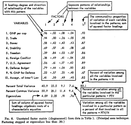
- The number of factors (columns) is the number of substantively meaningful independent (uncorrelated) patterns of relationship among the variables.28 Again considering the ten national characteristics, Figure 6 presents their unrotated matrix. As can be seen from the number of factors, there are four independent patterns of relationship in the data. These may be thought of as evidencing four different kinds of influence (causes) on the data, as presenting four categories by which these data may be classified, or as illuminating four empirically different concepts for describing national characteristics.
- The loadings, , measure which variables are involved in which factor pattern and to what degree (see Equation 1 and Equation 2).29 They can be interpreted like correlation coefficients (see Section 4.1). The square of the loading multiplied by 100 equals the percent variation that a variable has in common with an unrotated pattern.
One can look at this percent figure as the percent of data on a variable that can be produced or predicted by knowing the values of a case (such as a nation) on the pattern or on the other variables involved in the same pattern. Another perspective is that the percent figure is the reliability of prediction of a variable from the pattern or from the other variables in the same pattern. By comparing the factor loadings for all factors and variables, those particular variables involved in an independent pattern can be defined, and those variables most highly related to a pattern can also be seen.
For example, consider the unrotated factor loadings for the ten characteristics as shown in the first section of Table 3. Let a pattern be limited to those variables with 25 percent or more of their variation involved in a pattern (loading of .50, squared and multiplied by 100). Then the first pattern of interrelationships30 in Table 3 involves high GNP per capita (.96), trade (.94), power (.58), stability (.69), US agreement (.56), and defense budgets (.79).
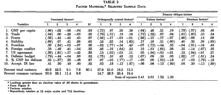
- The first unrotated factor pattern delineates the largest pattern of relationships in the data; the second delineates the next largest pattern that is independent of (uncorrelated with) the first; the third pattern delineates the third largest pattern that is independent of the first and second; and so on. Thus the amount of variation in the data described by each pattern decreases successively with each factor; the first pattern defines the greatest amount of variation, the last pattern the least. Note that unrotated factor patterns are uncorrelated with each other.31
- The column headed "h2" displays the communality of each variable. This is the proportion of a variable's total variation that is involved in the patterns. The coefficient (communality) shown in this column, multiplied by 100, gives the percent of variation of a variable in common with each pattern.
This communality may also be looked at as a measure of uniqueness. By subtracting the percent of variation in common with the patterns from 100, the uniqueness of a variable is determined. This indicates to what degree a variable is unrelated to the others--to what degree the data on a variable cannot be derived from (predicted from) the data on the other variables. In Table 3, for example, foreign conflict has a communality of .55. This says that 55 percent of the foreign conflict behavior as measured for the fourteen nations can be predicted from a knowledge of nation values on the four patterns; and that 45 percent of it is unrelated to the other nine characteristics.
The h2 value for a variable is calculated by summing the squares of the variable's loadings. Thus for power in Table 3 we have (.58)2 + (-.42)2 + (-.42)2 + (.43)2 = .87, the h2 value.
- The ratio of the sum of the values in the h2 column to the number of variables, multiplied by 100, equals the percent of total variation in the data that is patterned. Thus it measures the order, uniformity, or regularity in the data. As can be seen in Table 3, for the ten national characteristics the four patterns involve 80.1 percent of the variation in the data. That is, we could reproduce 80.1 percent of the relative variation among the fourteen nations on these ten characteristics by knowing the nation scores on the four patterns.
- At the foot of the factor columns in Figure 6, the percent of total variance figures show the percent of total variation among the variables that is related to a factor pattern. This figure thus measures the relative variation among the fourteen nations in the original data matrix that can be reproduced by a pattern: it measures a pattern's comprehensiveness and strength.
The sum of these figures for each pattern equals the sum of the column of h2 multiplied by 100. Looking along the row of percent of total variance figures and up the column of h2, one can see how the order in the data is divided by pattern and by variable.
The percent of total variance figure for a factor is determined by summing the column of squared loadings for a factor, dividing by the number of variables, and multiplying by 100.
- The percent of common variance figures indicate how whatever regularity exists in the data is divided among the factor patterns. The percent of total variance figures, discussed above, measure bow much of the data variation is involved in a pattern; the percent ofcommon variance figures measure how much of the variation accounted for by all the patterns is involved in each pattern. These latter figures are calculated in the same way as the percent of total variance, except that the divisor is now the sum of the column of h2values, which measures the common variation among the data.
- The eigenvalues equal the sum of the column of squared loadings for each factor. They measure the amount of variation accounted for by a pattern. Dividing the eigenvalues either by the number of variables or by the sum of h2 values and multiplying by 100 determines the percent of either total or common variance, respectively, Often only the eigenvalues are displayed at the foot of factor tables.32
Not all factor studies present the h2 values or the percent of common or total variance. From the points just made, however, the reader should be able to calculate them himself. In conjunction, information on the factor loadings and on communalities should enable the reader to relate the findings in an unrotated matrix to his particular concerns.
The rotated factor matrix should not differ in format from the unrotated factor matrix, except that the h2 may not be given and eigenvalues are inappropriate.33
The unrotated factors successively define the most general patterns of relationship in the data. Not so with the rotated factors. They delineate the distinct clusters of relationships, if such exist. This is mentioned here to alert the reader to this difference. The distinction is clarified with illustrations in Section 5.
The following features characterize the rotated matrix:
- If the rotated matrix is orthogonal, that is mentioned in the title of the matrix (e.g., "orthogonally rotated factors"), or else the word varimax or quartimax appears in the title (these are techniques for orthogonal rotation). An orthogonally rotated matrix appears in the second section of Table 3, for the ten national characteristics of Table 1. The unrotated factor matrix from Figure 6 is also given for comparison (first section of Table 3). For an orthogonally rotated matrix the following aspects should be noted:
- Several features of the unrotated matrix are preserved by the orthogonally rotated matrix. These are the features described in Section 4.2 under the first point on the number of factors indicating the number of patterns, the second point on interpreting loadings, the sixth point on the percent of total variance, and the seventh point on the percent of common variance.
- The h2 values given for the unrotated factors do not change with orthogonal rotation, given the number of factors in each case is the same. Hence they may be given with either the unrotated or the rotated factor matrix.
- In the unrotated matrix, factor patterns are ordered by the amount of data variation they account for, with the first defining the greatest degree of relationship in the data. In the orthogonally rotated matrix, no significance is attached to factor order.
- Factors are uncorrelated (refer back to Note 31). For example, in Table 3, the first orthogonally rotated pattern--which might be labeled a power pattern--is uncorrelated with the second pattern, that of UN agreement with the US.
- If the rotated matrix is oblique rather than orthogonal, the title or description of the matrix will indicate this. The title may also contain strange terms like covarimin, quartimin, or biquartimin. These refer to various criteria for the rotation and need not trouble us here.
Oblique rotation means that the best definition of the uncorrelated and correlated cluster patterns of interrelated variables is sought. Orthogonal rotation defines only uncorrelatedpatterns; oblique rotation has greater flexibility in searching out patterns regardless of their correlation. This difference is elaborated with geometric illustrations in Section 5.
Oblique rotation takes place in one of two coordinate systems: either a system of primaryaxes or a system of reference axes. The reference axes give a slightly better definition of the clusters of interrelated variables than do the primary ones. For each set of axes there are two possible matrices: factor structure and factor pattern matrices. It is irrelevant to the consumer of factor results whether oblique primary or reference factors are given. There is an important difference, however, between the pattern matrix and the structure matrix.
- The primary factor pattern matrix and the reference factor structure matrix delineate the oblique patterns or clusters of interrelationship among the variables. Their loadings define the separate patterns and degree of involvement in the patterns for each variable. Unlike the unrotated or the orthogonally rotated factors, however, their loadings cannot be strictly interpreted as the correlation of a variable with a pattern, and the squared loadings do not precisely give the percent of variation of a variable involved in a pattern. Nevertheless, as in the orthogonal factor matrix, their loadings are zero when a variable is not involved in a pattern, and close to 1.0 when a variable is almost perfectly related to a factor pattern.34 The less correlated the oblique patterns are with each other, the more their loadings are like correlations of variables with patterns. With this understanding in mind, the reader mightroughly interpret the primary pattern matrix or reference structure matrix loadings as correlations. By squaring them and multiplying by 100 to get an idea of theapproximate percent of variation involved, the reader will have a conceptual anchor for understanding the configuration of loadings.
The third section of Table 3 displays the (primary) oblique pattern factor matrix for the ten national characteristics. These may be compared with the orthogonally rotated factors shown in the second section. Note how much more distinct the patterns are when defined by oblique rotation (the pattern matrix) than by orthogonal rotation. There are fewer moderate loadings and more high and low loadings, thus giving a better definition of the pattern of relationships.
- The primary factor structure matrix and the reference factor pattern matrix give the correlation of each variable with each pattern. The loadings are strictly interpretable as correlations. They can be squared and multiplied by 100 to measure the percent of variation of a variable accounted for by a pattern. The last section ofTable 3 shows the (primary) oblique structure factors matrix for the ten national characteristics. The basic difference between the primary structure and patternmatrices (or reference pattern and structure matrices) relevant for interpretation is that the primary pattern loadings best show what variables are highly involved in what clusters. The primary pattern loadings distinctly display the patterns. The primary structure loadings, however, do not display them well; instead, they measure the correlation of variables with the patterns. Note in Table 3 how much better the patterns among the ten national characteristics are differentiated by the pattern matrix loadings than by the structure matrix.
By this time, the many distinctions mentioned may have created more confusion than understanding. Table 4 shows the important differences for the several matrices considered. The difference between primary and reference matrices is one of geometric perspective. Reference matrices give a slightly better definition of the oblique patterns and are preferred by psychologists. Because of a simpler geometrical representation, however, I often use the primary matrices.

- The oblique factors will have a correlation among them as shown in a factor correlation matrix. This matrix is discussed in Section 4.4, below.
- Figures for percent of common variance and percent of total variance are not given for the oblique factors. In order to get some measure of the strength of the separate oblique factor patterns, the sum of a column of squared factor loadings may be computed. This has been done in Table 3 for the oblique factors for the ten national characteristics.
This is a correlation matrix between oblique factor patterns found through oblique rotation. Some studies may call this a matrix of factor cosines. The cosines, however, can be read as correlations between patterns, and vice versa. The characteristics of a correlation matrix described in Section 4.1 apply equally well here.
What does a nonzero correlation between two factors mean? It means that the data patterns themselves have a relationship, to the degree measured by the factor correlations. The idea that patterns can be related is not strange, since we continually deal with such notions in social theorizing. Weather patterns are related to transportation patterns, for example, and a modernization pattern is related to cultural patterns. Factor analysis makes these links explicit through oblique rotation and the factor correlation matrix.
Table 5 presents the factor correlations for the oblique factors shown in Table 1. From Table 5 it can be seen that voting agreement with the US and foreign conflict patterns are in fact orthogonal (uncorrelated) to each other. The foreign conflict pattern does have some positive relationship (.31) to the power pattern, however.
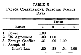
Sometimes the factor correlation matrix can itself be factor analyzed, as was the variable correlation matrix. This will uncover the pattern of relationships among the factors; the interpretation of these patterns does not differ from those found for the variable correlations. The reduction of factor interrelationships to their patterns is called higher order factor analysis.
The factor matrix presents the loadings , by which the existence of a pattern for the variables can be ascertained. The factor score matrix gives a score for each case (such as a nation) on these patterns.
The factor scores are derived in the following way: Each variable is weighted proportionally to its involvement in a pattern; the more involved a variable, the higher the weight. Variables not at all related to a given pattern--like the case of defense budget as percent of GNP, a variable unrelated to the orthogonally rotated first pattern in Table 3--would be weighted near zero. To determine the score for a case on a pattern, then, the case's data on each variable is multiplied by the pattern weight for that variable. The sum of these weight-times-data products for all the variables yields the factor score. Cases will have high or low factor scores as their values are high or low on the variables entering a pattern.35 For an economic development pattern involving GNP per capita, telephones per capita, and vehicles per capita, for example, the factor scores derived from the weighted summation of data of nations on these variables would place the United States as the highest, Japan as moderate, and Yemen near the bottom.
How are factor scores to be interpreted? Simply as data on any variable are interpreted. GNP as a variable, for example' is a composite of such variables as hog production, steel production, and vehicle production. Similarly, population is a composite of population subgroups. In the same fashion, factor scores on, say, an economic development pattern are a composite. The composite variables represented by factor scores can be used in other analyses or as a means of comparing cases on the patterns. But the factor scores have one feature that may not be shared by many other variables. They embody phenomena with a functional unity: the phenomena are highly interrelated in time or space.
Table 6 displays the factor scores for the fourteen nations on the (orthogonally rotated) four patterns of Table 3. These scores are standardized, which means they have been scaled so that they have a mean of zero and about two-thirds of the values lie between +1.00 and -1.00. Those scores greater than +1.00 or less than -1.00, therefore, are unusually high or low. Figure 2 plots these factor scores for the four patterns separately, and Figure 7 plots scores on the power and foreign conflict patterns against each other.
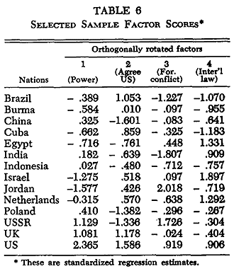
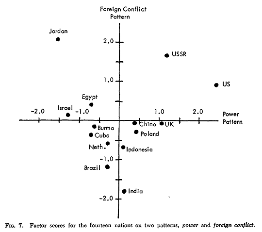
The loadings and factor scores describing the patterning of the data are found by the analysis. Once the patterns are determined, the scientist will study them and attach an appropriate label. These labels facilitate the communication and discussion of the results; they also serve as instrumental tags for further manipulation, mnemonic recall, and research. The scientist may label the patterns in any one of three ways: symbolically, descriptively, or causally.
Symbolic labels are simply any symbols without substantive meaning of their own. Their purpose is merely to denote the patterns. Three factor patterns, for example, may be labeled DI, D2, and D3, or A, B, and C. A label such as D, can be made equivalent to a given pattern without fear of adding surplus meaning. Alternatively, to name a pattern "economic development" or "totalitarianism" might have different connotations for different people.
Although symbolic tags are precise and help avoid confusion, they also create problems in communicating research findings and comparing studies. At the present stage of research in the social sciences, symbolic tags have yet to acquire agreed-on meanings reflecting a well-tested set of patterns, as has happened with vitamins (e.g., vitamin C).
By contrast, descriptive labels like "agreement with the US," once defined, can be easily remembered and referred to without redefinition. They are clues to factor content perhaps similar to those found by other studies. A descriptive interpretation of a pattern comprises selecting a concept that will reflect the nature of the phenomena involved. If, for example, a factor analysis of nations uncovers a pattern of intercorrelated data on total area, total population, total GNP, and magnitude of resources, the pattern might be named "size." The descriptive label is meant to categorize the findings.
In causal naming of patterns, the scientist reasons from the discovered patterns to the underlying influences causing them. The causal tag is a capsule explanation of why a pattern involves particular variables. For example, a factor pattern comprising coups and purges may be symbolically labeled "C," descriptively named "revolution," or causally termed "modernization." In the last case, the scientist may believe that the occurrence and intercorrelation among these revolutionary actions results from the social disruption of a rapid shift from a traditional society to a modem industrial nation. As another example, a factor analysis of Congressional roll call votes. may uncover a highly intercorrelated pattern of foreign policy issues. A descriptive label could be "foreign policy" pattern. Causally, however, it might be called an "isolationist" pattern by reasoning that a common isolationist attitude underlies the uniformity in foreign policy voting.
The approach to the interpretation of factor patterns is a matter of personal taste, communication, and long-run research strategy. The scientist may wish to use concepts that are congenial to the interests of the reader to facilitate communication, encourage thought about the findings, and make their use easier. There is always the danger, however, of the fallacy of misplaced concreteness. The interpretations of the findings within the research and lay community may be as much a result of the tag itself as of what the tag denotes.
5. FACTOR ROTATION
Almost all published factor analyses employ rotation. A section on rotation, therefore, may aid in comprehending the nature of the results. The character of the unrotated solution will be discussed first, and after that the nature and rationale for rotation.
5.1 Character of Unrotated Factors
For the most popular factor analysis techniques (centroid and principal axes), the factor patterns define decreasing amounts of variation in the data. Each pattern may involve all or almost all the variables, and the variables may therefore have moderate or high loadings for several factor patterns. To uncover the first pattern, a factor is fitted to the data to account for the greatest regularity; each successive factor is fitted to best define the remaining regularity. The result of this is that the first unrotated factor may be located between independent clusters of interrelated variables. These clusters cannot be distinguished in terms of their loadings on the first factor, although they will have loadings different in sign on the second and subsequent factors.
This situation may be illustrated in a two-factor, eight-variable case by Figure 8. Part (a) of this figure shows the eight hypothetical variables plotted according to their data for, say, 50 cases. These fifty cases are the coordinate axes of the space.36 As shown in Figure 8(b), the first factor, F1, falls between the two clusters of interdependent variables labeled I and II. In this position F1maximally reflects the variation of (i.e., has maximum loadings for) all eight variables. Another way of saying this is that the first factor lies along the center of gravity of all the points representing the variables. Observe that the separate loadings (dotted lines) of these variables on the first factor does not enable the clusters to be distinguished. Table 7 gives the factor loadings for the eight variables on unrotated F1.

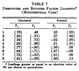
Figure 8(c) shows the variable loadings on the second factor, which is placed at right angles (orthogonal) to the first; Table 7 also gives these loadings on unrotated F2.
The first unrotated factor delimits the most comprehensive classification, the widest net of linkages, or the greatest order in the data. For comparative political data, a first factor could be a "political institutions" pattern, and a second might define the democratic and totalitarian poles. For international relations, the first factor could be participation in international relations, and a second factor might reflect a polarization between cooperation and conflict. For variables measuring heat, the first factor could be temperature and a second might delineate the extremes of hot and cold. For physiological measurements on adults, the first factor could be size and a second might mirror a polarization between height and girth.
5.2 Character of Rotated Factors
A scientist may rotate factors to see if a hypothesized cluster of relationships exists. This can be done by postulating the loadings of a hypothetical factor matrix and then rotating the factors to a best fit with this matrix. The truth of the hypothesis is tested by the difference between the fitted and hypothesized factor loadings.
Alternatively, a scientist may rotate the factors to control for certain influences on the results. He may rotate the first factor to a variable or group of variables and then rotate the subsequent factors to be at right angles (uncorrelated) with the first. This removes the effects of variables highly loaded on the first factor and enables us to assess the patterns independent of them.
Most often, however, a scientist rotates his factors to a simple structure solution. When a factor matrix is entitled "rotated factors," this almost always means a simple structure rotation. That is, each factor has been rotated until it defines a distinct cluster of interrelated variables. Through this rotation the factor interpretation shifts from unrotated factors delineating the most comprehensive data patterns to factors delineating the distinct groups of interrelated data.
Consider again the unrotated factors shown in Figure 8(c). A simple structure rotation would be equivalent to that shown in Figure 9. The new factor positions F*1 and F*2 now clearly distinguish the two clusters. This rotated factor matrix is shown in Table 7 alongside the unrotated factors.

A simple structure rotation has several characteristics of interest here:
- Each variable is identified with one or a small proportion of the factors. If the factors are viewed as explanations, causes, or underlying influences, this is equivalent to minimizing the number of agents or conditions needed to account for the variation of distinct groups of variables.
- The number of variables loading highly on a factor is minimized. This changes the unrotated factor patterns from being general to the largest number of variables to patterns involving separate groups of variables. The rotation attempts to define a small number of distinct clusters of interrelated phenomena. The simple structure type of matrix is illustrated in Table 8. The moderate and large factor loadings are indicated by x and small loadings are left blank.
- A major ontological assumption underlying the use of simple structure is that, whenever possible, our model of reality should be simplified. If phenomena can be described equally well using simpler factors, then the principle of parsimony is that we should do so. Simple structure maximizes parsimony by shifting from general factors involving all the variables to group factors involving different sets of variables.
- A goal of research is to generalize factor results. The unrotated factor solution, however, depends on all the variables. Add or subtract a variable from the study and the results are altered. The unrotated solution should be adjusted, then, so that the factors will be invariant of the variables selected. An invariate factor solution will delineate the same clusters of relationships regardless of the extraneous variables included in the analysis.
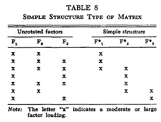
One of the chief justifications for simple structure rotation is that it determines invariant factors. This enables a comparison of the factor results of different studies. Very seldom do different scientists study exactly the same variables. But when variables overlap between studies and each study employs simple structure rotation, tests can be made to see if the same patterns are consistently emerging.
5.3 Orthogonal Simple Structure Rotation
One important type of simple structure rotation is an orthogonal one. A second type is oblique simple structure (discussed in Section 5.4 below). Factors rotated to orthogonal simple structure are usually reported simply as "orthogonal factors." Occasionally, the varimax or quartimaxcriteria for achieving the rotation are used to designate the factors.
Orthogonality is a restriction placed on the simple-structure search for the clusters of interdependent variables. The total set of factors is rotated as a rigid frame, with each factor immovably fixed to the origin at a right angle (orthogonal) to every other factor. This system of factors is rotated around the origin until the system is maximally aligned with the separate clusters of variables. If all the clusters are uncorrelated with each other, each orthogonal factor will be aligned with a distinct cluster. The more correlated the separate clusters are, however, the less clearly can orthogonal rotation discriminate them. Simple structure can then only be approximated, not achieved.
Whether or not uncorrelated clusters of relationship exist in the data, orthogonal rotation will still define uncorrelated patterns of relationships. These patterns may not completely overlap with the distinct clusters, but the delineation of these uncorrelated factors is useful. Results involving uncorrelated patterns are easier to communicate, and the loadings can be interpreted as correlations. Moreover, orthogonal factors are more amenable to subsequent mathematical manipulation and analysis.
5.4 Oblique Simple Structure Rotation
Whereas in orthogonal simple structure rotation the final factors are necessarily uncorrelated, in oblique rotation the factors are allowed to become correlated. In orthogonal rotation the whole factor structure is moved around the origin as a rigid frame (like the spokes of a wheel around the hub) to fit the configuration of clusters of interrelated variables. In oblique rotation to simple structure, however, the factors are rotated individually to fit each distinct cluster. The relationship between the resulting factors then reflects the relationship between the clusters.Figure 10(a) shows a two-factor orthogonal simple structure rotation; for comparison, Figure 10(b) displays a simple structure oblique rotation to the same clusters.37

Orthogonal rotation is a subset of oblique rotations. If the clusters of relationships are in fact uncorrelated, then oblique rotation will result in orthogonal factors. Therefore, the difference between orthogonal and oblique rotation is not in discriminating uncorrelated or correlated factors but in determining whether this distinction is empirical or imposed on the data by the model.
Controversy exists as to whether orthogonal or oblique rotation is the better scientific approach. Proponents of oblique rotation usually advocate it on two grounds:
- it generates additional information; there is a more precise definition of the boundaries of a cluster, and the central variables in a cluster can be identified by their high loadings;
- the correlations between the clusters are obtained, and these enable the researcher to gauge the degree to which his data approximate orthogonal factors.
Besides yielding more information, oblique rotation is justified on epistemological grounds. One justification is that the real world should not be treated as though phenomena coagulate in unrelated clusters. As phenomena can be interrelated in clusters, so the clusters themselves can be related. Oblique rotation allows this reality to be reflected in the loadings of the factors and their correlations. A second justification is that correlations between the factors now allow the scientific search for uniformity to be carried to the second order (see Section 4.4). The factor correlations themselves may be factor analyzed to determine the more general, the more abstract, the more comprehensive relationships and the more pervasive influences underlying phenomena.
NOTES
* Scanned from "Understanding Factor Analysis," The Journal of Conflict Resolution (December 1967): 444-480. Typographical errors have been corrected, clarifications added, and style updated. This was an invited paper prepared in connection with research supported by the National Science Foundation, GS-1230. For many helpful comments made on a draft of that published, I wish to thank Henry Kariel, Michael Haas, Robert Hefner, Woody Pitts, and J. David Singer. This article is a summary of Rummel (1970).
1. Note omitted.
2. For a bibliography of applications of factor analysis in the social sciences (excluding psychology), see Rummel (1970). A bibliography of applications to conflict and international relations is given in the appendix below.
3. How many readers know that over a decade ago Raymond Cattell (1949) gave us the first comprehensive findings on the extent to which foreign and domestic conflict behaviors have been correlated with many socioeconomic and political characteristics of nations?
4. For a Q-factor analysis of UN voting, see Russett (1966). A Q-factor analysis of nations on many of their characteristics has been reported by Banks and Gregg (1965).
5. Most factor analysis done on nations has been R-factor analysis. As one example out of many, see Tanter (1966). R- and Q-factor analyses do not exhaust the kinds of patterns that may be considered. Other possible patterns of variation are those in characteristics over time units for a specified nation (this identifies similar time periods); in nations over time units for a characteristic (this identifies nations similarly changing on a characteristic); and in time units over nations for a characteristic ( this identifies similar time periods for nations changing on a characteristic). For a discussion of these varieties of analysis, see Rummel (1970, Chapter. 8).
6. Section 4.2 discusses how such percentage figures are derived from the factor results.
7. For example, see Borgatta and Cottrell's classificatory work on groups (1955) and Schuessler and Driver's on tribes (1956). Selvin and Hagstrom (1963) show, through an example, how to use factor analysis to develop a classification of groups. Using factor analysis, Russett classifies nations into their regional groups (1967) and their UN voting blocs (1966).
8. For practical applications of this two-step design, see Buckatzsch ( 1947) and Berry (1960).
9. On this and related points, see the particularly excellent Chapters 19 and 20 in Cattell (1952). Cattell (1966) has recently elaborated the position that factor analysis is, among other things, an experimental method.
10. See the discussion on the relationship between hypotheses and factor analysis in Cattell (1952, pp. 13-14). For an application of factor analysis to test a hypothesis about the supposed dimensions of urban areas, see van Arsdol, Camilleri, and Schmid (1958).
11. An extended discussion of description and explanation with regard to factor analysis in psychology is given by Henrysson (1957). Thurstone (1947, Chapter 6) discusses factors as explanatory concepts in terms of a demonstration problem involving the dimensions of cylinders. His illustration of this problem is helpful for understanding factor analysis in practice.
12. The distinction being drawn here is between descriptive and inferential statistics, not between description and statistics.
13. Some of the more excellent treatments are those by Frank (1955, Chapter 1), Kaufmann (1958, Chapter 6), the essays by Russell, Feigl, and Nagel in Part V of Feigl and Brodbeck (1953), and Nagel (1961).
14. "It would seem that in general the variables highly loaded in a factor are likely to be the causes of those which are less loaded, or at least that the most highly loaded measures--the factor itself--is causal to the variables that loaded on it" (Cattell, 1952, p. 362). Cattell and Sullivan (1962) conducted a demonstration experiment by factoring data on cups of coffee to determine whether patterns corresponding to known causal influences could be delineated. They found a strong correlation between the known patterns of influences and those defined by the factor analysis. With like results a similar experiment was conducted on the dynamics of balls (Cattell and Dickman, 1962). These artificial experiments are helpful in understanding applied factor analysis.
15. Positive empirical evidence for this view is referred to in Note 14.
16. See the clear and explicit analysis by Abel (1953) of the operation of verstehen in the social sciences.
17. One of the best discussions of theory is given by Nagel (1961, Chapter 6). That theory construction consists of two parts is argued by Einstein. See the essays on Einstein's philosophy by Frank, Lenzen, and Nortbrup in Schilpp (1949).
18. An exciting theoretical use of factor analysis has been published by Cattell. (1962). He describes a role behavior model potentially rooted in empirical data, tying together personality, structure, and syntal group dimensions. A theoretical embodiment of factor analysis to relate the attributes and behavior of social units is described in Rummel (1965).
19. The relationship between classical physics and quantum theory, or between Cartesian analysis and Hilbertian analysis as related to factor analysis, is discussed by Ahmavaara (Ahmavaara and Markkanen, 1958, pp. 48-63). This analysis is the most refreshing and provocative that I have read on the subject. See also Note 25, below.
20. Prior to plotting, the data would have to be made comparable through some standardization procedure.
21. The cosine of this angle between vectors is, with minor qualifications, equal to the product moment correlation coefficient between the characteristics represented by the vectors. Thus, a correlation of 1.00 between two variables on twenty cases means that the angle is zero between the two vectors (variables) plotted in the space of twenty dimensions (cases).
22. I am referring to the results of the factor analysis research design, which include the application of a factoring technique plus simple structure rotation. (See Section 5.2) For those familiar with linear algebra, it may be helpful to know that a factor analysis defines a set of basis dimensions for the column vectors of a data matrix. Each basis dimension of a rotated set uniquely generates an independent subset of the original vectors. The basis dimensions of an unrotated set are ordered by their contributions to generating all the vectors.
23. The configuration of vectors in Figure 5 is four-dimensional. Therefore, although the placement of the two independent axes is the best (orthogonal) definition of the two clusters in four-dimensional space, the two-dimensional figure can only display this fit imperfectly.
24. This is where curve-fitting techniques like multiple linear and curvilinear regression analysis are helpful.
25. The factor analysis model has much in common with quantum theory. This is one reason I have argued, as I do in Section 2.5 above, that factor analysis is a theoretical structure as well as a data analysis technique. See Margenau (1950, Chapter 17) for a clear and simple description of quantum theory. Burt (1941) and Ahmavaara in Ahmavaara and Markkanen (1958) have also drawn the comparison of factor analysis with quantum theory.
26. Confusion on this score has caused much unfounded criticism of factor analysis as delineating only linear relationships.
27. The idea of a correlation coefficient gives another perspective on factor analysis. The patterns discovered by a factor analysis consist of those variables highly intercorrelated. Thus, if variable A is highly correlated with both B and C, and if B and C are highly correlated with each other, then A, B, and C form a correlation cluster. If A, B, and C are not correlated with other variables, then they form an independent pattern that factor analysis will delineate.
28. There is some question about the criteria for determining the exact number of factor patterns for a set of data. Variation in the number of patterns defined by different criteria is usually small and, at any rate, normally concerns the minor patterns. The larger patterns, involving many variables with high loadings, will ordinarily be found and reported regardless of the criteria employed.
29. Note how the organization of a factor matrix is like the layout of Equation 1. Rather than explicitly organizing the factor results in equations, factor analysts use the matrix format, where the first column refers to the F1 function, the second column to the F2 function, etc., and the elements (loadings) of the matrix are the constants, , that have been found by the analysis.
30. These patterns differ from those given as examples for these variables in Section 1. This is because we are now discussing unrotated patterns. The reason for the differences will be discussed below.
31. To say the factors are uncorrelated means that the factor scores (to be discussed in Section 4.5) on the factor patterns are uncorrelated, and not necessarily the factor loadings. Factor loadings are, however, independent (orthogonal)
32. The eigenvalues are extracted only if the principal axes method of factor analysis is used. An eigenvalue is the root of the characteristic equation [R -  I] = 0, where R is the correlation matrix, is an eigenvalue, I is an identity matrix, and the brackets mean that the determinant is being computed. Let X be an orthogonal matrix with columns determined such that XR = X. Then the various roots, , are the eigenvalue solutions to the equation and X is the matrix of eigenvectors. The factor matrix is equal to the eigenvectors times the reciprocal square root of their associated eigenvalues.
33. Although equal to the sum of squared factor loadings, the eigenvalue is technically a solution of the characteristic equation (see Note 32) for the unrotated factors. The rotated factors are derived from these by transformation (rotation).
34. The pattern matrix loadings are best understood as regression coefficients of the variables on the patterns.
35. These factor scores then give values for each case on the functions, F, of Equations 1, 2, and 3in Section 3.2. With the constant, , defined by the factor matrix, and the factor scores defining the value of the function, F, the factor equations are completely specified.
36. At this point the reader may find it helpful to review Section 3.1.
37. Various mathematical criteria are employed to achieve oblique simple structure, and have such exotic names as quartimin, covarimin, biquartimin, binormin, promax, and maxplane.These may sometimes appear in the title of an oblique factor matrix.
REFERENCES
Abel, Theodore. "The Operation Called Verstehen." In Herbert Feigl and May Brodbeck (eds.),Readings in the Philosophy of Science. New York: Appleton Century Crofts, 19n.
Ahmavaara, Yrjö, and Tourco Markkanen. The Unified Factor Model. The Finnish Foundation for Alcohol Studies, 1958.
Alker, Hayward, Jr. "Dimensions of Conflict in the General Assembly." American Political Science Review, 58 (1964), 642-57.
________ and Bruce Russett. World Politics in the General Assembly. New Haven, Conn.: Yale University Press, 1965.
Banks, Arthur S., and Phillip M. Gregg. "Grouping Political Systems: Q-Factor Analysis of 'A Cross-Polity Survey,'" American Behavioral Scientist, 9 (1965), 3-6.
BERRY, Brian J. L. "An Inductive Approach to the Regionalization of Economic Development." In Norton Ginsburg (ed.), Essays on Geography and Economic Development. Chicago: University of Chicago Press, 1960.
Borgatta, E. F., and L. S. Cottrell, Jr. "On the Classification of Groups," Sociometry, 18 (1955), 665-678.
Buckatzsch, E. J. "The Influence of Social Conditions on Mortality Rates," Population Studies, 1 (1947), 229-48.
Burt, C. The Factors of the Mind. New York: Macmillan, 1941.
Cattell, Raymond B. Factor Analysis. New York: Harper Brothers, 1952.
________. "Group Theory, Personality and Role: A Model for Experimental Researches." In F. A. Geldard (ed.), NATO Symposium an Defense Psychology. New York: Pergamon Press, 1962.
________. "Multivariate Behavioral Research and the Integrative Challenge," Multivariate Behavioral Research, 1 (Jan. 1966), 4-23.
________. "The Dimensions of Culture Patterns by Factorization of National Characters,"Journal of Abnormal and Social Psychology, 44 (1949), 443-469.
________, and K. Dickman. "A Dynamic Model of Physical Influences Demonstrating the Necessity of Oblique Simple Structure," Psychological Bulletin, 59 (1962), 3894M.
________, and William Sullivan. "The Scientific Nature of Factors: A Demonstration by Cups of Coffee," Behavioral Science, 7 (1962), 184-93.
Ezekiel, Mordecai, and Karl A. Fox. Methods of Correlation and Regression Analysis, 3rd Edition. New York: Wiley and Sons, 1959.
Feigl, Herbert, and May Brodbeck (eds.). Readings in the Philosophy of Science. New York: Appleton Century Crofts, 1953.
Frank, Philip. Modern Science and its Philosophy. New York: Braziller, 1955.
Hanson, Norwood Russell. "On the Symmetry Between Explanation and Prediction," The Philosophical Review, 68 (1959), 349-58.
Hempel, Carl G. Aspects of Scientific Explanation and Other Essays in the Philosophy of Science. New York: Free Press, 1965.
________. "Fundamentals of Concept Formation in Empirical Science." International Encyclopedia of Unified Science, 2. Chicago: University of Chicago Press, 1952.
Henrysson, Sten. Applicability of Factor Analysis in the Behavioral Sciences. Stockholm: Almqvist and Wiksell, 1957.
Kaufmann, Felix. Methodology of the Social Sciences. New York: Humanities Press, 1958.
Margenau, Henry. The Nature of Physical Reality. New York: McGraw-Hill, 1950.
Nagel, Ernest. The Structure of Science. New York: Harcourt, Brace and World, 1961.
Rummel, R. J. "A Field Theory of Social Action with Application to Conflict Within Nations."General Systems Yearbook, 10 (1965), 183-211.
________. Applied Factor Analysis. Evanston, ILL: Northwestern University Press.
________. "Some Attribute and Behavioral Patterns of Nations," Journal of Peace Research, 2 (1967), 196-206.
________. The Dimensions of Nations. Beverly Hills, CA: Sage Publications, 1972.
Russett, Bruce. "Delineating International Regions." In J. David Singer (ed.), Quantitative International Politics. Glencoe: Free Press, 1967.
________. "Discovering Voting Groups in the United Nations," American Political Science Review, 60 (June 1966), 327-39.
Schilpp, Paul Arthur (ed.). Albert Einstein: Philosopher-Scientist. Evanston: Library of Living Philosophers, 1949.
Schuessler, K. F., And Harold Driver. "A Factor Analysis of Sixteen Primitive Societies,"American Sociological Review, 21 (1956), 493-9.
Selvin, Hanan C., And Warren 0. Hagstrom. "The Empirical Classification of Formal Groups,"American Sociological Review, 28 (1963), 399-411.
Tanter, Raymond. "Dimensions of Conflict Behavior Within and Between Nations, 1958-60,"Journal of Conflict Resolution, 10 (March 1966), 41-64.
Thurtstone, L. L. Multiple-Factor Analysis. Chicago: University of Chicago Press, 1947.
Van Arsdol, Maurice D., Jr., Santo F. Camilleri, and Calvin F. Schmid. "The Generality of Urban Social Area Indexes," American Sociological Review, 23 (1958), 277-84.
APPENDIX
BIBLIOGRAPHY OF FACTOR ANALYSIS
IN CONFLICT AND INTERNATIONAL STUDIES
Adelman, Irma, and Cynthia T. Morris. "Factor Analysis of the Interrelationship Between Social and Political Variables and Per Capita Gross National Product," Quarterly Journal of Economics,79, (Nov. 1965), 555-78.
Alker, Hayward, Jr. "Dimensions of Conflict in the General Assembly," American Political Science Review, 58 (1964), 642-57.
________. "Supranationalism in the United Nations," Peace Research Society: Papers III, 1965, Peace Research Society (International) Chicago Conference, 1964.
________, and Bruce M. Russett. World Politics in the General Assembly. New Haven, Conn.: Yale University Press, 1965.
Banks, Arthur S., and Phillip Gregg. "Grouping Political Systems: Q-Factor Analysis of 'A Cross-Polity Survey,' " American Behavioral Scientist, 9 ( 1965), 3-6.
Berry, Brian J. L. "An Inductive Approach to the Regionalization of Economic Development." In Norton Ginsburg (ed.), Essays on Geography and Economic Development. Chicago: University of Chicago Press, 1960.
________. "Basic Patterns of Economic Development." In Norton Ginsburg (ed.), Atlas of Economic Development. Chicago: University of Chicago Press, 1961, 110-19.
Cattell, Raymond B. "A Quantitative Analysis of the Changes in Culture Pattern of Great Britain, 1837-1937, by P-Technique," Acta Psychologica, 9 (1953), 99-121.
________. "The Dimensions of Culture Patterns by Factorization of National Characters,"Journal of Abnormal and Social Psychology, 44 (1949), 443-69.
________. "The Principal Culture Patterns Discoverable in the Syntal Dimensions of Existing Nations," Journal of Social Psychology, 32 (1950), 215-53.
________. and Marvin Adelson. "The Dimensions of Social Change in the U.S.A. as Determined by P-Technique," Social Forces, 30 (1951), 190-201.
________, H. Breul, and H. P. Hartman. "An Attempt at More Refined Definitions of the Cultural Dimensions of Syntality in Modern Nations," American Sociological Review, 17 (1952), 408-21.
________, and Richard L. Gorsuch. "The Definition and Measurement of National Morale and Morality," Journal of Social Psychology, 67 (1965), 77-96.
Chadwick, Richard W. Developments in a Partial Theory of International Behavior: A Test and Extension of Inter-Nation Simulation Theory, Ph.D. dissertation, Northwestern University, 1966.
Denton, Frank H. "Some Regularities in International Conflict, 1820-1949," Background, 9 (Feb. 1966), 283-96.
Feierabend, Ivo K., and Rosalind L. "Aggressive Behaviors Within Polities, 1948-1962: A Cross-National Study," Journal of Conflict Resolution, 10, 3 (Sept. 1966), 249-71.
Gibb, Cecil A. "Changes in the Culture Pattern of Australia, 1906-1946, as Determined by the P-Technique," Journal of Social Psychology, 43 (1956), 225-38.
Gregg, Phillip M., and Arthur S. Banks. "Dimensions of Political Systems: Factor Analysis of 'A Cross-Polity Survey,'" American Political Science Review, 59 (Sept. 1965), 602-14.
Hatt, Paul K., Nellie L. Farr, and Eugene Weinstein. "Types of Population Balance," American Sociological Review, 20, 1 (Feb. 1955), 14-21.
Laulicht, Jerome. "An Analysis of Canadian Foreign Policy Attitudes," Peace Research Society: Papers III, 1965, Peace Research Society (International) Chicago Conference, 1964.
McClelland, C., et al. The Communist Chinese Performance in Crisis and Non-Crisis: Quantitative Studies of the Taiwan Straits Confrontation, 1950-64. Final Report of Completed Research under contract for Behavioral Sciences Group, Naval Ordnance Test Station, China Lake, Calif. (N60530-11207), Dec. 14, 1965.
Megee, Mary. "Problems in Regionalization and Measurement," Peace Research Society: Papers IV, 1966, Peace Research Society (International), Cracow Conference (1965), 7-35.
Morris, Charles. Varietics of Human Value. Chicago: University of Chicago Press, 1956.
Rummel, R. J. "A Field Theory of Social Action with Application to Conflict Within Nations,"General Systems Yearbook, 10 1965), 183-211.
________. "A Social Field Theory of Foreign Conflict," Peace Research Society: Papers IV, 1966, Peace Research Society (International), Cracow Conference, 1965a.
________. "Dimensions of Conflict Behavior Within and Between Nations," General Systems Yearbook, 8 (1963), 1-50.
________. "Dimensions of Conflict Behavior within Nations, 1946-1959," Journal of Conflict Resolution, 10, 1 (March 1966), 65-73.
________. "Dimensions of Dyadic War, 1820-1952," Journal of Conflict Resolution, 11, 2 (June 1967), 176-83.
________. "Dimensions of Foreign and Domestic Conflict Behavior: Review of Findings." In Dean Pruitt and Richard Snyder (eds.), Theory and Research on the Causes of War. Englewood Cliffs, N.J.: Prentice-Hall, 1969.
________. "Some Attribute and Behavioral Patterns of Nations," Journal of Peace Research, 2 (1967), 196-206.
________. "Some Dimensions in the Foreign Behavior of Nations," Journal of Peace Research,3 (1966), 201-24.
________. Dimensions of Nations. Santa Barbara, CA: Sage Publications, 1972.
Russett, Bruce M. "Delineating International Regions." In J. David Singer (ed.), Quantitative International Polities. Glencoe: Free Press, 1968.
________. "Discovering Voting Groups in the United Nations," American Political Science Review, 60 (June 1966), 327-39.
________ International Regions and International Integration. Chicago: Rand McNally, 1967.
Schnore, Leo F. "The Statistical Measurement of Urbanization and Economic Development,"Land Economics, 37, 3 (Aug. 1961), 229-45.
Tanter, Raymond. "Dimensions of Conflict Behavior \\1ithin Nations, 1955-1960: Turmoil and Internal War," Peace Research Society: Papers III, 1965, Peace Research Society (International) Chicago Conference, 1964.
________. "Dimensions of Conflict Behavior Within and Between Nations, 1958-60," Journal of Conflict Resolution, 10 (March 1966), 41-64.
Subscribe to:
Posts (Atom)